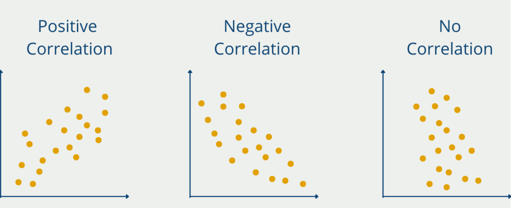
Correlation refers to the relationship between two statistical variables. The two variables are then dependent on each other and change together.  A positive correlation of two variables, therefore, means that an increase in A also leads to an increase in B. The association is undirected. It is therefore also true in the reverse case and an increase in variable B also changes the slope of A to the same extent.

Causation, on the other hand, describes a cause-effect relationship between two variables. Causation between A and B, therefore, means that the increase in A is also the cause of the increase in B. The difference quickly becomes clear with a simple example:

A study could likely find a positive correlation between a person’s risk of skin cancer and the number of times they visit the outdoor pool. So if a person visits the outdoor pool frequently, their risk of developing skin cancer also increases. A clear positive association. But is there also a causal effect between outdoor swimming pool visits and skin cancer? Probably not, because that would mean that only outdoor swimming pool visits are the cause of the increased risk of skin cancer.

It is much more likely that people who spend more time in outdoor swimming pools are also exposed to significantly more sunlight. If they do not take sufficient precautions with sunscreen or similar, more sunburns can occur, which increases the risk of skin cancer. The correlation between outdoor swimming pool visits and skin cancer risk is not causal. 

A variety of curious correlations that very likely do not show causation can be found at tylervigen.com.

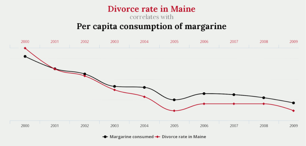
For example, there is a very high association between the divorce rate in the American state of Maine and the per capita consumption of margarine. Whether this is also causation can be doubted.

What are the Types of Correlation?

In general, two types of contexts can be distinguished:

1. Linear or Non-Linear: The dependencies are linear if the changes in variable A always trigger a change with a constant factor in variable B. If this is not the case, the dependency is said to be non-linear. For example, there is a linear correlation between height and body weight. With every new centimeter of height gained, one is very likely to also gain a fixed amount of body weight, as long as one’s stature does not change. A non-linear relationship exists, for example, between the development of sales and the development of a company’s share price. With a 30% increase in sales, the stock price may increase by 10%, but with the subsequent 30% increase in sales, the stock price may only increase by 5%.
2. Positive or Negative: If the increase in variable A leads to an increase in variable B, then there is a positive correlation. If, on the other hand, the increase in A leads to a decrease in B, then the dependency is negative.

How is the Pearson correlation calculated?

To calculate the Pearson correlation coefficient, the following steps are usually performed:

1. Calculations of the means for both variables.
2. Calculations of the standard deviation for both variables.
3. Deviation from the mean: For each of the two variables and for each element in the data set, the deviation from the respective mean is calculated. It is important to note that this is done element by element.
4. Multiplying the deviations: For each pair of deviations from the mean, the product is then calculated and summed.
5. Dividing by standard deviation: This result is finally divided by the product of the two standard deviations and the number of observations, which was reduced by one.

In short form, the corresponding formula looks as follows:

\(\) \[r = \frac{ \sum_{i \in D}((x_{i} – \text{mean}(x)) \cdot (y_{i} – \text{mean}(y))}{((n-1) \cdot SD(x) \cdot SD(y)}\]

where:

• Σ represents across all observations in the datasets.
• xi and yi are the individual observations for variables x and y.
• mean(x) and mean(y) are the mean values for variables x and y.
• SD(x) and SD(y) are the individual standard deviations.
• n is the number of observations and n-1 correspondingly the number reduced by one.

What is the (Pearson) Correlation Coefficient and how is it interpreted?

The Correlation Coefficient indicates how strong the association between the two variables is. In the example of tylervigen.com, this correlation is very strong at 99.26% and means that the two variables move almost 1 to 1, i.e. an increase in the consumption of Margarine by 10% also leads to an increase in the divorce rate by 10%. This is illustrated in the screenshot above, as margarine consumption and the divorce rate decrease almost in parallel. This shows that a decrease in margarine consumption also leads to a decrease in the divorce rate.

The coefficient can also assume negative values. A coefficient smaller than 0 describes the Anti-Correlation and states that the two variables behave in opposite ways. For example, a negative association exists between current age and remaining life expectancy. The older a person gets, the shorter his or her remaining life expectancy. 

What role does correlation play in Machine Learning?

Correlation plays an important role in machine learning. It helps in identifying the relationships between the features and the target variable in the dataset. The correlation coefficient measures the degree of relationship between two variables. Machine learning algorithms use correlation to identify patterns and dependencies between features in the data.

There are several types of measures such as Pearson’s coefficient, Spearman’s rank coefficient, and Kendall’s tau coefficient that can be used in Machine Learning models.

The correlation between the features and the target variable can help in selecting the relevant features for the model. If two features are highly correlated, one of them can be removed from the model as it does not provide any additional information. This process is called feature selection.

Correlation can also help determine the direction of the relationship between the characteristics and the target variable. For example, a positive correlation between age and income means that as age increases, the income also increases. This information can help make predictions or recommendations based on the input data.

However, it is important to note that correlation is not the same as causality. Machine learning models should not assume causality just because two variables are highly correlated. It is necessary to conduct experiments or randomized controlled trials to establish a causal relationship between variables.

Therefore, while correlation is an important Machine Learning tool, it should be used in combination with other statistical methods and techniques to ensure accurate and reliable predictions.

What are the pitfalls and fallacies about correlation and causation?

When researching relationships between variables, it is important to be aware of common pitfalls and fallacies that can occur. Understanding these pitfalls can help researchers and analysts avoid misinterpretations and incorrect conclusions. The following are some of the most common pitfalls:

A common mistake is the fallacy that correlation implies causation. It is incorrect to assume that a correlation between two variables implies a causal relationship. Correlation measures the statistical relationship between variables, but does not establish causality. Additional evidence and rigorous study designs are needed to establish causality.

Another pitfall is reverse causality, in which the assumed cause and effect can be reversed. The erroneous assumption of the direction can lead to incorrect interpretations. Thorough analysis and temporal considerations are necessary to establish the correct causal relationship.

Confounding variables present another challenge. These are third variables that can influence both the presumed cause and effect. Failure to account for confounding variables can lead to spurious correlations and misleading conclusions. Careful study design and statistical techniques such as multivariate analysis can help identify and control for confounding variables.

The post hoc fallacy is a common misconception in which it is assumed that a correlation implies causality simply because of the timing of events. Just because one event precedes another does not necessarily mean that it caused the subsequent event. Other factors, coincidences, or common causes may contribute to the observed relationship.

Another phenomenon to note is the Simpson paradox. It occurs when a correlation observed within subgroups of data reverses or disappears when the groups are combined. This highlights the importance of considering subgroup analysis and the potential impact of hidden factors that may influence the relationship between variables.

The ecological fallacy is an error that occurs when conclusions are drawn about individuals based on group-level correlations. Assumptions about individuals based solely on aggregate data can lead to erroneous conclusions. To avoid this fallacy, individual-level data should be considered.

Another pitfall to watch out for is the omitted variable bias. The omission of relevant variables in the analysis can lead to bias and affect the observed correlation. It is important to include all relevant factors and potential confounders in the analysis to mitigate this bias.

To effectively avoid these pitfalls and confounders, critical thinking, rigorous study designs, consideration of alternative explanations, and replication of results are essential.

How do you prove Causation?

To reliably prove causation, scientific experiments are conducted. In these experiments, people or test objects are divided into groups (you can read more about how this happens in our article about Sampling), so that in the best case all characteristics of the participants are similar or identical except for the characteristic that is assumed to be the cause.

For the “skin cancer outdoor swimming pool case”, this means that we try to form two groups in which both groups of participants have similar or preferably even the same characteristics, such as age, gender, physical health, and exposure to sunlight per week. Now it is examined whether the outdoor swimming pool visits of one group (note: the exposed sun exposure must remain constant), changes the skin cancer risk compared to the group that did not go to the outdoor swimming pool. If this change exceeds a certain level, one can speak of causation.

Why are experiments important for proving causality?

The importance of experiments and randomized controlled trials (RCTs) in proving causality cannot be overstated. Here are some reasons why:

• Control: with an experimental design, researchers can control for any confounding factors that might affect the outcome variable. In an RCT, participants are randomly assigned to a treatment or control group, ensuring that any differences in outcomes can be attributed to the intervention and not to pre-existing differences between groups.
• Replication: the use of experiments and RCTs allows the replication of results by other researchers. This helps establish the robustness of the results and the generalizability of the intervention.
• Accuracy: By controlling for all possible confounding variables, experiments, and RCTs can provide more accurate estimates of causal effects.
• Ethical considerations: In some cases, it may be unethical to establish causation through observational studies alone. For example, it would be unethical to observe the effects of a harmful drug on pregnant women without first testing it in an RCT.
• Policy Implications: Evidence of causality is essential for informed policy decisions. Without experimental evidence, policymakers could make decisions based on correlations alone, leading to ineffective or harmful policies.
• Scientific Progress: Finally, experiments and RCTs are essential for scientific progress. They allow researchers to test hypotheses, refine theories, and develop new interventions that can improve people’s lives.

In summary, experiments and RCTs are essential to demonstrate causality and improve our understanding of complex phenomena in fields such as medicine, psychology, and economics. While observational studies can provide valuable information, they should be viewed as a complement to experimental research, not a substitute.

This is what you should take with you

• Only in very few cases does a correlation also imply causation.
• Correlation means that two variables always change together. Causation, on the other hand, means that the change in one variable is the cause of the change in the other.
• The correlation coefficient indicates the strength of the association. It can be either positive or negative. If the coefficient is negative, it is called anticorrelation.
• To prove a causal effect one needs complex experiments. 

Other Articles on the Topic of Correlation and Causation

• Detailed definitions of the terms can be found here.