Pandas and Numpy are the most basic libraries when it comes to data manipulation in Python. This post gives insight into the most important basics in this library and can also be used as a cheat sheet for the most common commands.

Pandas brings all the tools needed for any form of data manipulation and analysis. With the help of special data structures, table-like objects and time series data can be stored and processed. Pandas builds in many cases on Numpy and is therefore not in competition with this library, as is sometimes claimed.

What is Pandas?

Pandas is a high-performance, open-source data manipulation and analysis library for Python. Designed to make data wrangling and analysis seamless, it provides a powerful set of tools built on top of the Python programming language. Whether you’re handling small datasets or massive dataframes, this library empowers you to efficiently manipulate, clean, and analyze structured data, making it an essential toolkit for data scientists, analysts, and enthusiasts.

Why Pandas?

• User-Friendly Syntax: Pandas adopts an intuitive and expressive syntax, making it accessible for both beginners and experienced programmers.
• Community Support: With a large and active community, the module benefits from continuous improvement, updates, and a wealth of online resources, tutorials, and forums for troubleshooting.
• Versatility: From exploratory data analysis to complex statistical modeling, Pandas is a versatile tool that adapts to various stages of the data science workflow.

In essence, Pandas is your go-to companion for taming the complexities of data. Whether you’re preparing data for machine learning models, conducting statistical analyses, or exploring datasets for insights, it equips you with the tools to efficiently handle the challenges of data manipulation in Python.

How can you install and set up Pandas?

To begin your journey with Pandas, start by ensuring a seamless installation and setup process. If you haven’t already installed Python on your system, head to the official Python website at python.org/downloads. During installation, be sure to check the option to “Add Python to PATH.”

Once Python is installed, open a terminal or command prompt and run the command pip install pandas to fetch and install the latest version of Pandas from the Python Package Index (PyPI).

To verify the successful installation, open a Python interpreter or a Jupyter Notebook and type the following:

This should display the installed version, confirming that it’s ready for use.

If you’re using Jupyter Notebooks, you can install Pandas directly within the notebook by running the command !pip install pandas. For Anaconda users, Pandas is often pre-installed, but you can update it using conda install -c anaconda pandas.

With Pandas successfully installed, create a new Python script or notebook in your preferred environment, whether it’s a code editor like VSCode or an integrated environment like Jupyter Notebooks. Include the import statement import pandas as pd at the beginning of your script to start using it in your projects.

Consider using an Integrated Development Environment (IDE) like VSCode or PyCharm for an enhanced coding experience, offering features like code completion, debugging, and interactive data exploration.

With Pandas now part of your Python toolkit and your environment ready, you’re poised to explore the vast capabilities of Pandas for efficient data manipulation and analysis.

Which Data Structures are available in Pandas?

Pandas is characterized by two central data structures that make it a powerful tool for data manipulation and analysis: the Series and the DataFrame.

Series:

The Series is a one-dimensional, labeled data structure in Pandas. Similar to a column in a table or a single variable in statistics, the Series offers flexible data handling. Each entry in the Series is uniquely identified by an index, facilitating efficient selection and manipulation.

Example of a Series:

DataFrame:

The DataFrame is a two-dimensional, table-like data structure. It consists of multiple columns, with each column being a Series. The DataFrame allows efficient organization and manipulation of structured data. Like the Series, the DataFrame is characterized by an index that enables the unique identification of rows.

Example of a DataFrame:

Key Features:

• Flexibility: Both the Series and the DataFrame can accommodate data of different types, including numeric, textual, or time-based data.
• Efficient Indexing: The index allows for quick selection, filtering, and manipulation of data in Pandas DataFrames.
• Diverse Operations: These data structures enable a variety of operations, including filtering, sorting, grouping, aggregating, and more.
• Integration with Numpy and Matplotlib: Pandas seamlessly integrates with NumPy for numeric operations and Matplotlib for data visualization.

Mastering these data structures empowers you to leverage the full spectrum of Pandas for complex data analyses and manipulations. Whether it’s filtering datasets, merging tables, or creating meaningful visualizations, these data structures form the core of your data exploration.

What is the difference between a Python list and a NumPy array?

At this point in the article, you might think that NumPy arrays are simply an alternative to Python lists, which even have the disadvantage of only being able to store data of a single data type, whereas lists also store a mixture of strings and numbers. However, there must be reasons why the developers of NumPy have decided to introduce a new data element with the array.

The main advantage of NumPy arrays over Python Lists is the memory efficiency and associated speed of reads and writes. In many applications this may not really matter, however, when dealing with millions or even billions of elements, it can offer significant time savings. Thus, arrays are often used in complex applications to develop high-performance systems.

What are the basic operations in Pandas?

When working with structured data in Pandas, mastering basic operations is crucial. These operations, applicable to both Series and DataFrame, form the bedrock of efficient data manipulation and analysis.

1. Data Loading:

Importing data into Pandas is seamless. Utilize read_csv(), read_excel(), or other data input methods to load data from various sources, such as CSV files or Excel sheets.

2. Data Inspection:

Understanding your dataset is key. Utilize methods like head(), tail(), info(), and describe() to gain quick insights into the structure, types, and summary statistics of your data.

3. Selection and Indexing:

Efficiently select data based on conditions or specific criteria. Leverage boolean indexing for precise data extraction.

4. Sorting Data:

Arrange your data based on specific columns or indices using sort_values().

5. Missing Values Handling:

Identify and handle missing values using methods like isnull(), dropna(), or fill missing entries using fillna().

6. Grouping and Aggregation:

Group your data based on certain criteria using groupby(). Apply aggregate functions like sum(), mean(), or custom functions to grouped data.

7. Data Visualization:

Integrate Pandas seamlessly with visualization libraries like Matplotlib and Seaborn. Create insightful plots directly from your data.

Mastering these fundamental operations provides you with the toolkit to explore, clean, and analyze datasets efficiently. As you delve deeper into your data exploration journey, these operations serve as the building blocks for more advanced analyses and insights.

How can you create objects in Pandas?

Pandas uses different data structures to store and process information. Unfortunately, we cannot go into detail about the different structures in this article and therefore refer to our other articles, e.g. about Pandas DataFrames.

Series

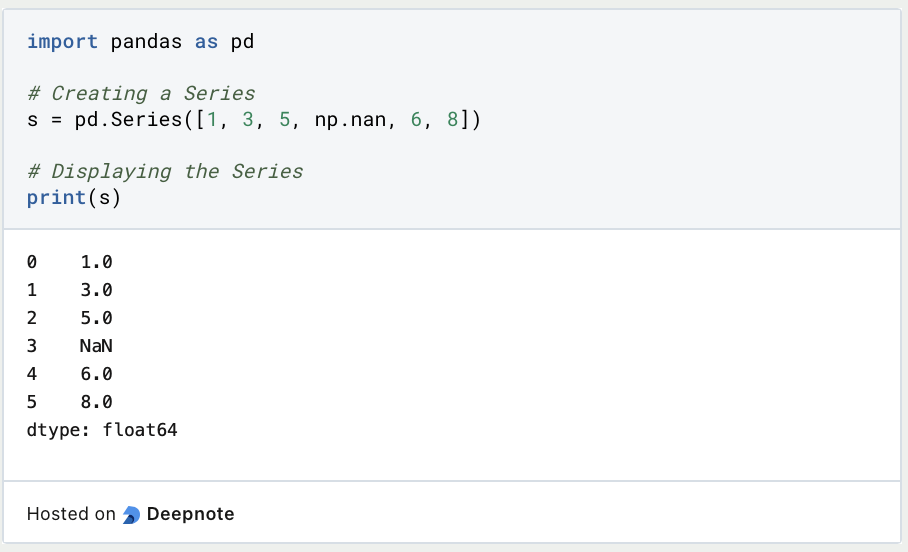
The Pandas Series object is similar to the one-dimensional Numpy Array and can hold various data structures, such as integers, floats, or strings.

In the output, we see two columns, although we have only defined values for the Series. The left column is the index, which by default numbers the values. We can access the index and the values with the following commands.

Of course, we can also define the index freely, making it easier and more understandable to access the elements by index. This also makes the code easier to read if you use talking text for access instead of numbers.

DataFrame

For a detailed explanation of DataFrames and many code examples, feel free to read our separate post on Pandas DataFrames. Here we will show only the most basic commands for the sake of completeness.

We can create a DataFrame by passing a Numpy array and defining the column names. We can call the individual rows of the table via the index, similar to the Series.

How can you view data?

We can view the first and last rows of a DataFrame with the following commands. In parentheses, we specify the number of rows we want to have an output from. The default value is five.

If we want to get a brief statistical overview of the data in each column, we can do that with df.describe():

In addition, we can also look at the data sorted directly by specifying the column name by whose values we want to sort.

How can you select Data?

Our execution in this chapter also applies to Panda’s Series objects with a few exceptions, so we will spare the examples for Series objects. We can select a column of the DataFrame by calling the name directly.

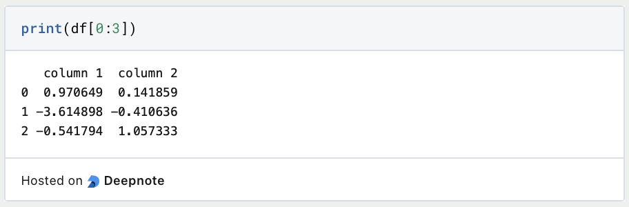
We call individual lines of the DataFrame either via the desired numbering or via the indexes/names we have assigned to them.

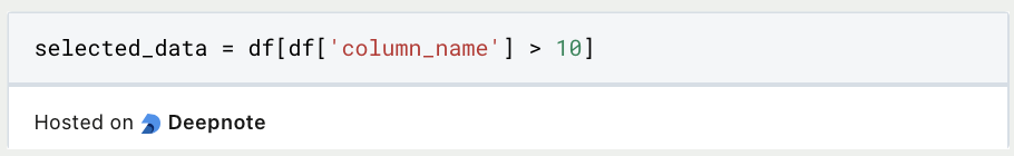
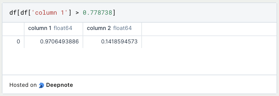
If we want to filter only the values that meet a certain condition, we define the column and the value that must be met. We have to keep in mind that in Python conditions with the equal sign, always need a double equal sign.

That should be it with a short introduction to the most basic commands in Pandas. The second part will follow in a few days.

How can you use Pandas for Data Visualization?

Data visualization is a powerful aspect of Pandas, seamlessly integrating with popular libraries like Matplotlib and Seaborn. This integration allows you to effortlessly create insightful visualizations directly from your dataset. Below is a guide to help you unlock the potential of data visualization using Pandas:

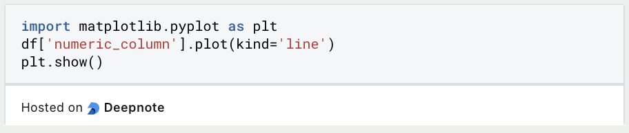
1. Line Plots:
Visualizing trends over time or continuous data becomes simple with line plots. Pandas’ plot() method streamlines the process, providing a quick way to generate such visualizations.

For example, you can create a line plot for a numeric column:

2. Histograms:
Examine the distribution of numeric data with histograms. This visualization method offers a rapid overview of data patterns and the presence of outliers.

For instance, you can create a histogram for a numeric column:

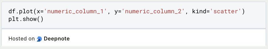
3. Scatter Plots:
Explore relationships between two numeric variables using scatter plots. This type of visualization is useful for identifying correlations between variables.

Here’s an example of creating a scatter plot:

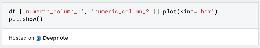
4. Box Plots:
Detect statistical outliers and understand data distribution through box plots. This visualization method provides valuable insights into the spread of your data.

For instance, you can create a box plot for selected numeric columns:

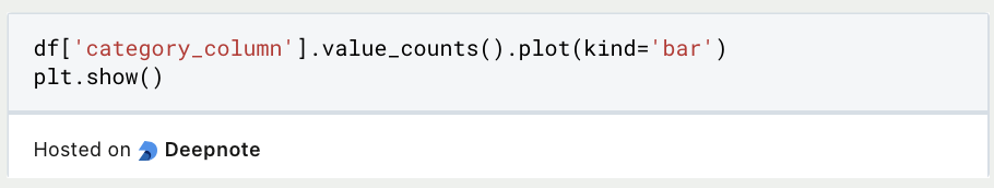
5. Bar Plots:
Visualize categorical data or compare quantities across different categories using bar plots. This type of visualization is effective for representing counts or proportions.

For example, you can create a bar plot for a categorical column:

6. Pie Charts:
Represent the proportion of different categories in your dataset using pie charts. This type of visualization is suitable for displaying the distribution of categorical data.

For instance, you can create a pie chart for a categorical column:

7. Customizing Plots:
Tailor your visualizations by customizing plot parameters, such as colors, labels, and titles. This allows you to create visualizations that effectively convey your insights.

As an example, you can customize a line plot with specific colors and labels:

Pandas, in conjunction with Matplotlib and Seaborn, simplifies the process of creating meaningful visualizations. This enables you to communicate your data insights effectively, turning your dataset into compelling visual narratives. Whether you’re exploring trends, distributions, or relationships, Pandas provides the tools to transform your data into engaging and informative visuals.

This is what you should take with you

• Pandas empowers efficient data manipulation and analysis with an expressive syntax.
• Accommodating diverse data types, Pandas’ Series and DataFrame offer flexibility and efficiency.
• The module seamlessly integrates with Matplotlib and Seaborn for creating insightful visualizations.
• Basic operations like loading, inspection, and sorting are foundational for exploration.
• Pandas simplifies identifying and handling missing data with methods like dropna().
• Grouping and aggregation operations extract statistical insights from data.
• It facilitates effective communication of insights through various plot types.
• Pandas offers a vast array of functionalities, encouraging continuous learning.
• Proficiency in Pandas opens the gateway to advanced data analysis and manipulation.
• The Pandas community and documentation contribute to a supportive learning environment.

Other Articles on the Topic of Pandas

• The official documentation of Pandas can be found here.
• This post is mainly based on the tutorial from Pandas. You can find it here.