The Markov chain is a central concept in mathematics and stochastics and is used to predict the probability of certain states in stochastic processes. The central feature of such systems is the so-called “memorylessness”, since the probability of each event depends only on the current state of the system and not on the past.

In this article, we take a closer look at the central properties of the Markov chain and go into the mathematical representation in detail. We also talk about real examples and simulate such a state model in Python.

What is the Markov chain?

A Markov chain is a central model in probability theory that deals with sequences of random events. The central feature of this chain is that each probability of an event depends exclusively on the state the system is currently in. The previous events, on the other hand, are completely irrelevant for the probability of the next step. More precisely, a Markov chain is a process that satisfies the Markov property, as it states that the future behavior of a system does not depend on the past, but only on the current state.

A classic example of a Markov chain is the game Monopoly. Several players move across the playing field with a roll of the dice. On each turn, the probability of the future square depends solely on the dice roll and the player’s current square. However, how the player arrived at the current square no longer plays a role in future behavior.

What terms are used in connection with the Markov chain?

Before we can delve deeper into the mathematical definition of Markov chains, we need to introduce some terms that are used in the field of probability calculation in general and in the field of Markov chains in particular. The most important terms and concepts include

State space

The state space is defined as the set of all possible states that a system can assume in a Markov chain. Each element in this state space describes a specific situation in which the system can find itself at any given time. However, it is not necessarily the case that this state is actually reached during the course of the system. This state space can comprise both a finite number of states and an infinite number of states.

Examples:

• A simple weather model, for example, only predicts the values “sun” or “rain”. Thus, the state space comprises a set of two states and is expressed as {rain, sun}.
• In Monopoly or any other board game, the state space includes all the squares that can be reached during the game. Although a square represents a possible state in the course of the game, it is not guaranteed that this square will actually be reached in a game.
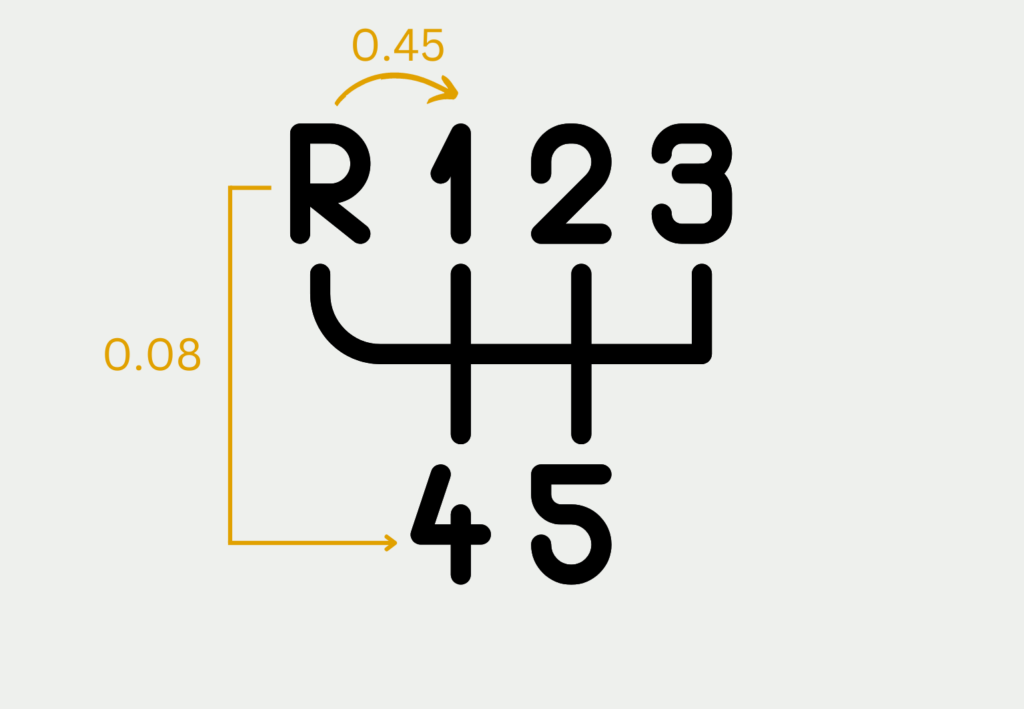
• In a gearshift car, the state space of the gearbox includes all gears that are available, for example {reverse gear, 1st gear, 2nd gear, 3rd gear, 4th gear, 5th gear}.

Transition Probability / Transition Matrix

The transition probability describes the probability that the system will transition from one state to another at a given point in time. In the Markov chain, this probability depends exclusively on the current state of the system due to the Markov property and not on the past of the system. When shifting gears, for example, these probabilities can be such that it is significantly more likely to change from reverse gear to first gear.g zu schalten als vom Rückwärtsgang in den vierten Gang. 

All transition probabilities that can be assumed in the next state are recorded in the transition matrix. All transition probabilities in a row must add up to 1 to ensure that a state is taken next. Mathematically, the transition matrix \(P\) for \(n\) states is described using a \(n \times n\) matrix in which the element \(p_{i,j}\) indicates the probability of transitioning from state \(i\) to state \(j\).

\(\) \[ P = \begin{pmatrix}
p_{R,R} & p_{R,1} & 0 & 0 & 0 & 0 \\
p_{1,R} & p_{1,1} & p_{1,2} & 0 & 0 & 0 \\
0 & p_{2,1} & p_{2,2} & p_{2,3} & 0 & 0 \\
0 & 0 & p_{3,2} & p_{3,3} & p_{3,4} & 0 \\
0 & 0 & 0 & p_{4,3} & p_{4,4} & p_{4,5} \\
0 & 0 & 0 & 0 & p_{5,4} & p_{5,5}
\end{pmatrix} \]

This also results in a transition matrix for the gear change, whereby we assume that no gears can be skipped and, for example, that it is only possible to downshift from third gear to second gear or upshift to fourth gear. There is also the possibility of remaining in third gear, which is described by the probability \(p_{3,3}\).

Discrete Markov chain

In a discrete Markov chain, the states are only changed at specific, discrete points in time. This means that the system only changes at predefined points in time and typically at equal intervals. In the Monopoly game, for example, the system playing field only ever changes during a turn.

Continuous Markov chain

In continuous Markov chains, the state changes occur at random points in time that lie continuously on a time axis. This means that the time of a transition is purely random and depends on a probability distribution. When driving a gearshift car, for example, the gear changes do not take place at fixed points in time, but depend on the traffic flow and the speed being driven. As a result, they are subject to a probability distribution.

With the help of these basic concepts and terms, we can now define a Markov chain in general mathematical terms.

What does the mathematical representation of the Markov chain look like?

A Markov chain is described mathematically by its own transition matrix \(P\), which can be defined in general terms as follows:

\(\)\[P(X_{n+1} = j \mid X_n = i) = p_{ij} \]

Here \(p_{ij}\) is generally the probability that a system transitions from the state \(i\) to the state \(j\). The transition matrix comprises all possible states that the system can assume, i.e. that lie in the state space.

In addition, the transition matrix is stochastic, which in turn means that all entries of the matrix in a row add up to one, so that the system will certainly transition to a new state after each step or remain in the current state. This fact is expressed mathematically as follows:

\(\) \[\sum_{j} p_{i,j} = 1 \]

What properties does a Markov chain have?

Markov chains have several important properties that determine the behavior and dynamics of the chain. The following describes some of the properties that a Markov chain can, but does not have to have.

Irreducibility

A Markov chain is irreducible if all transition probabilities are true positive, i.e. non-zero and non-negative. This property means that it is possible to reach a different state from any state in the system. The gear shifting example only becomes irreducible if it is possible to skip gears and thus shift directly from reverse gear to sixth gear.

Periodicity

A state is periodic if it is only possible to reach the state again after a period of \(d\) steps. Although the system remains stochastic, there is a certain determinism. In Monopoly, for example, the periodic property is expressed by the fact that you can return from the starting point to the starting point, but a certain minimum number of moves is required to do so, as you have to move around the entire field once.

Stationary distribution

A Markov chain follows a stationary distribution if there is a starting distribution that does not change over the course of the system and therefore remains stationary. Mathematically, this distribution is described by \(\pi\). This has the property that if \(\pi\) is multiplied by the transition matrix \(P\), the distribution \(\pi\) is obtained again:

\(\) \[\pi \cdot P = \pi \]

By solving this equation, the stationary distribution and a fixed probability for each transition can be found.

Recurrence and Transcendence

These properties revolve around the long-term behavior of Markov chains and describe how often certain states are reached. If a state is visited almost infinitely often in the long-term behavior, then it is called recurrent. Otherwise it is called transient. If all states in a state space are recurrent, then the entire Markov chain is called recurrent.

What is the long-term behavior of Markov chains?

The focus of the analysis of Markov chains is on how the system behaves in the long term and whether there is a state to which the system converges and what the probabilities then look like in this equilibrium. Central to the analysis of long-term behavior is the equilibrium state and absorbing states.

A central aspect of Markov chains is the equilibrium state or the stationary distribution. Under certain circumstances, the Markov chain converges to this distribution after sufficient steps. The stationary distribution is the distribution which, when multiplied by the transition matrix, results in the distribution.

In Monopoly, for example, the system tends towards a stationary distribution in the long term, which describes how often the players have been on the various squares. In this case, the prison square or the starting square has a higher probability than the other squares, as there are several ways to get to these squares.

Another important observation in the long-term behavior of Markov chains is whether so-called absorbing states occur. These states are reached when the system is no longer able to leave this state and therefore remains there. In gambling, for example, the absorbing state is reached when a player no longer has any money and can therefore no longer participate in the game of chance.

What special types of Markov chains are there?

Markov chains are general stochastic models that can already be used to simulate many real processes. However, there are also applications that are not compatible with the properties presented so far. For this reason, various special Markov chains have been developed over time.

Birth and death processes are used to describe continuous Markov chains that experience state changes through discrete events. The process models how individuals suddenly appear or disappear in the system. These can be used for an online store, for example, when new users appear or leave the online store. The transition probabilities then describe the frequency with which such birth or death processes take place.

With reversible Markov chains, it is not clear whether the process runs forwards or backwards. The process can therefore be reversed without the transition probabilities changing. Simply put, this means that the probability of transitioning from state \(i\) to state \(j\) is just as high as transitioning from state \(j\) to state \(i\).

These special chains are mainly used in physics and chemistry when modeling equilibrium systems. Due to the mathematical properties, mathematical simplifications can be made.

How can a Markov chain be simulated and implemented in Python?

In practical application and analysis, the simulation of Markov chains is particularly interesting in order to investigate the long-term properties and behavior of these systems and to draw conclusions about reality. Markov chains are used in various fields, such as the natural sciences or financial mathematics.

One widely used option for this is the so-called Monte Carlo simulation. This involves repeatedly generating random sequences of states and thus estimating the statistical properties of the chain. In general, these steps are repeated:

1. Initialization: First, a starting state is selected from which the system begins.
2. Transition: The transition probabilities are used to determine the next state in the system.
3. Repetition: Step 2 is repeated several times to simulate a longer period of time.
4. Statistical analysis: After this time, the frequency of the states can be considered in order to estimate the stationary distribution or other properties of the Markov chain.

Using this approach, the Markov chain can be analyzed quickly and easily without the need for an analytical solution of the transition equations.

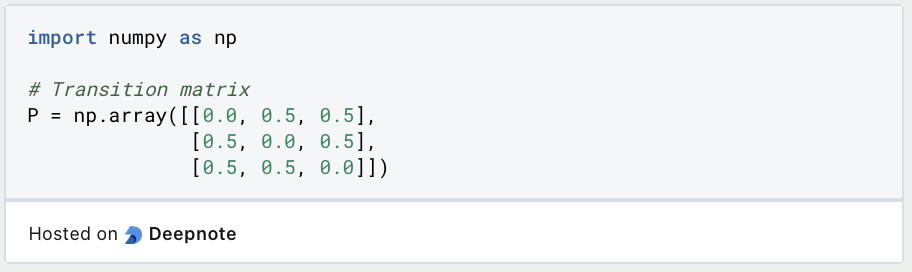
To illustrate this approach in Python, we use a fictitious Markov chain with a total of three states. We define the transition probabilities in such a way that the probability of changing from one state to another is 50%. To ensure that the probabilities in one row of the transition matrix are 100%, the probability that the Markov chain remains in the same state is 0%. In Python, this transition matrix can be created using a NumPy array.

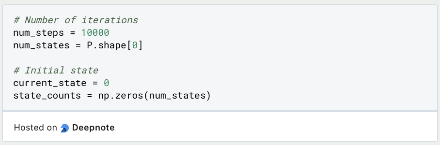
Next, the system is initialized and the initial state is defined. We also repeat the Monte Carlo simulation 10,000 times.

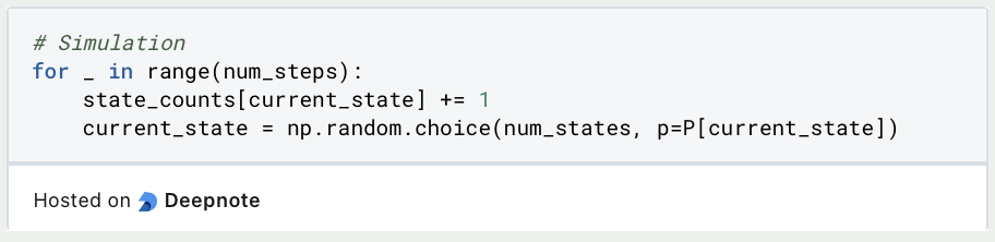
During the simulation, one of the three states is randomly selected in each step and then advanced to. The probabilities from the transition matrix are taken into account.

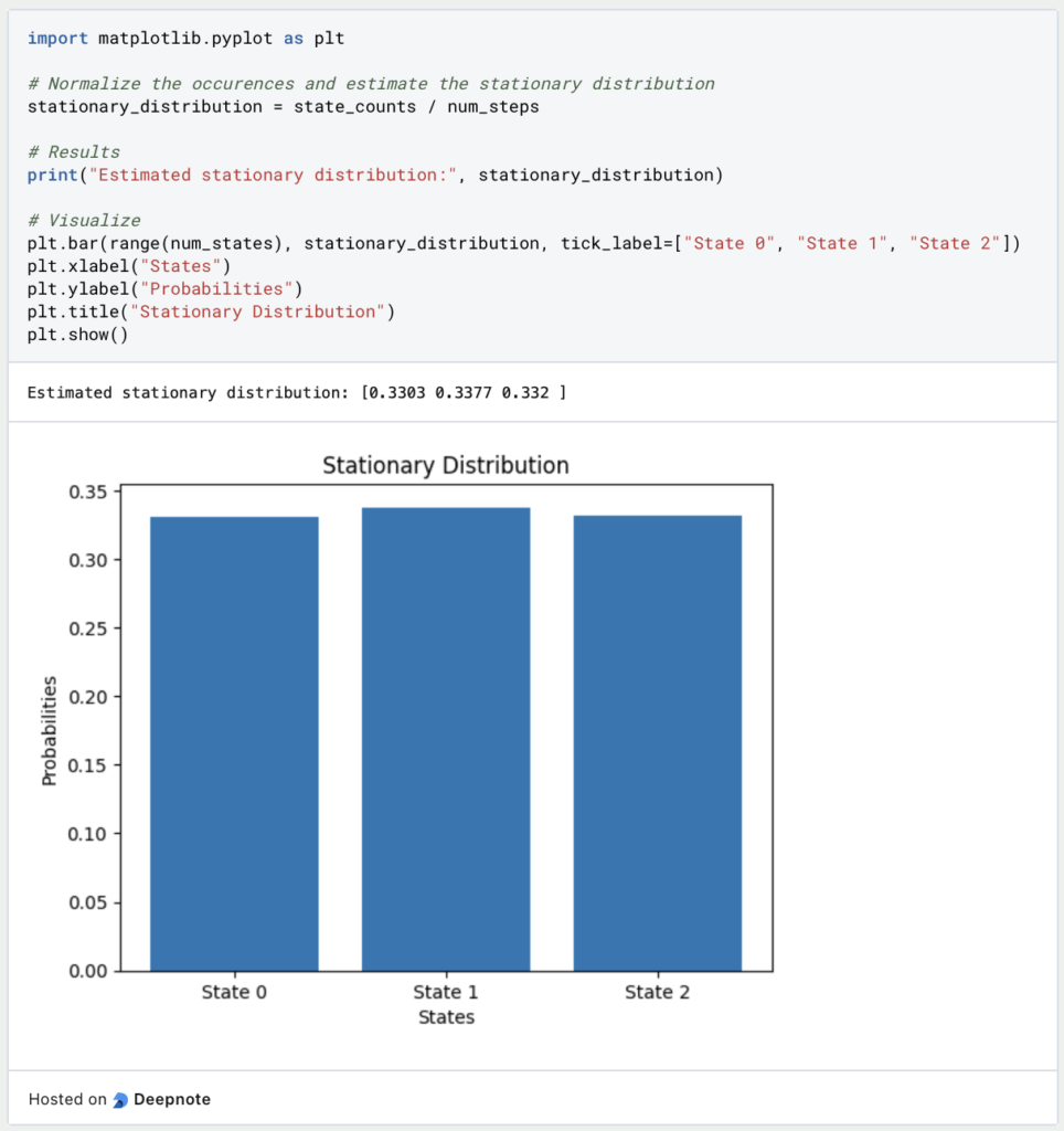
Finally, we can now calculate the stationary distribution and display it graphically using Matplotlib. As expected, the three states are almost equally likely. With the help of more repetitions, this picture would become even more solid:

This is what you should take with you

• Markov chains are stochastic models that describe systems of states and how they behave over a period of time.
• The Markov property applies to these chains, which states that the probability of the next state depends solely on the current state of the system and not on the past.
• Depending on the time definition, there are continuous and discrete Markov chains.
• Markov chains can have different properties, such as periodicity or recurrence.
• To simulate Markov chains, the so-called Monte Carlo simulation is often used, which can also be easily implemented in Python.

Other Articles on the Topic of the Markov Chain

The University of Ulm has a script about Markov Chains that you can find here.