Monte Carlo methods, often referred to simply as Monte Carlo simulations, are a powerful and versatile class of computational techniques used to solve a wide range of complex problems. These methods are named after the Monte Carlo Casino in Monaco, known for its games of chance, as they rely on randomness and probabilistic sampling to approximate solutions to problems that may be deterministic or stochastic in nature. Monte Carlo methods have found applications across diverse fields, from physics and finance to statistics and machine learning, making them an indispensable tool in the toolkit of scientists, engineers, analysts, and researchers.

In this article, we will embark on a journey to explore the fascinating world of Monte Carlo methods. We will delve into the principles that underlie these techniques, understand how they leverage random sampling, and discover their effectiveness in solving problems that were once considered intractable. From estimating complex integrals to optimizing financial portfolios, from training sophisticated machine learning models to unraveling the mysteries of quantum physics, Monte Carlo methods offer a flexible and efficient approach to tackle a multitude of challenges.

What are Monte Carlo Methods?

Monte Carlo methods represent a fascinating and versatile class of computational techniques with applications spanning numerous fields, including finance, physics, engineering, and statistics. These methods are rooted in the core concept of randomness and are designed to provide approximate solutions to problems that are often too complex or impractical to solve using traditional analytical methods. Exploring the basics of Monte Carlo methods is akin to opening a gateway to the world of probabilistic problem-solving.

At its heart, Monte Carlo draws its inspiration from randomness. The name itself is an homage to the renowned Monte Carlo Casino in Monaco, famous for games of chance, underscoring the central role of randomness in these techniques. In Monte Carlo simulations, randomness is harnessed as a tool to estimate intricate quantities, explore diverse scenarios, or tackle challenging problems.

Monte Carlo simulations typically commence with the generation of random samples or inputs. These samples are often drawn from specific probability distributions that capture the inherent uncertainty within the problem’s context. Each random sample corresponds to a potential state or scenario within the system or model under examination.

A fundamental application of Monte Carlo methods is numerical integration. Rather than relying on traditional calculus-based approaches for calculating definite integrals, Monte Carlo approximations leverage random sampling. The idea is to scatter random points within the integration domain and compute the average function value over these points. This average serves as an estimation of the integral, particularly useful for functions with complex analytical solutions.

Monte Carlo techniques are particularly adept at simulating complex systems or processes. By introducing random inputs or variations into a system, one can estimate its behavior or characteristics. This includes the determination of expected outcomes, assessment of variances, or computation of probabilities associated with different scenarios.

The strength of Monte Carlo methods lies in their remarkable flexibility and broad applicability. They shine in situations where obtaining analytical solutions proves challenging, costly, or infeasible. Monte Carlo methods excel in addressing problems characterized by uncertainty, variability, or inherent randomness.

Monte Carlo methods find application across an array of fields and disciplines, showcasing their versatility:

• Finance: They aid in assessing investment risks, pricing financial derivatives, and optimizing portfolios.
• Physics: Monte Carlo simulations are employed for simulating particle interactions, modeling quantum systems, and understanding the behavior of complex physical systems.
• Engineering: These methods are used for analyzing the reliability of structures and systems, conducting probabilistic risk assessments, and optimizing engineering designs.
• Statistics: In the realm of statistics, Monte Carlo Markov Chain (MCMC) techniques are employed for Bayesian inference, and simulations play a pivotal role in statistical studies.
• Computer Graphics: Monte Carlo methods facilitate the rendering of realistic images by simulating the behavior of light and materials, leading to the creation of visually stunning computer graphics.

As you delve further into the realm of Monte Carlo methods, you’ll discover not only their prowess in approximating solutions but also their ability to introduce a probabilistic dimension to problem-solving. The elegance of Monte Carlo simulations lies in their adaptability, making them valuable for both theoretical exploration and practical problem-solving in a multitude of domains.

How does the Monte Carlo Simulation work?

The Monte Carlo simulation method operates on the principles of randomness, statistical sampling, and numerical approximation. It’s essentially a process of conducting experiments or computations using random input values to estimate the behavior, characteristics, or outcomes of a system, process, or problem. Here’s a step-by-step explanation of how the Monte Carlo simulation works:

1. Define the Problem: Start by clearly defining the problem you want to solve or the system you want to model. This could be anything from estimating the value of a complex integral to simulating the behavior of financial markets.
2. Identify Input Variables: Determine the input variables or parameters that influence the problem. These could be factors like interest rates, material properties, initial conditions, or any other relevant parameters.
3. Specify Probability Distributions: For each input variable, specify a probability distribution that represents its uncertainty or variability. Common distributions include uniform, normal (Gaussian), exponential, or custom distributions tailored to the problem.
4. Generate Random Samples: Using the specified probability distributions, generate a large number of random samples for each input variable. These samples represent potential values for the variables, capturing the uncertainty inherent in the problem.
5. Run Simulations: For each combination of random samples, run the simulation or computation that models the problem. This may involve solving equations, simulating physical processes, or conducting other relevant computations.
6. Collect Data: Record the outcomes or results of each simulation run. This could be the solution to an equation, the behavior of a physical system, or any other relevant data.
7. Analyze Results: After running a sufficient number of simulations, you’ll have a dataset of results. Analyze this dataset to draw conclusions about the problem. Common analyses include computing averages, variances, percentiles, or other relevant statistics.
8. Estimate the Solution: Use the statistical properties of the collected data to estimate the solution or make predictions about the system. For example, if you were estimating the value of a complex integral, the average of the computed results from the simulations can serve as an estimate.
9. Assess Accuracy: Determine the level of accuracy and confidence in your estimated solution. This may involve calculating confidence intervals, conducting sensitivity analyses, or assessing convergence.
10. Repeat as Needed: Depending on the desired level of accuracy, you can repeat the simulation with more random samples or iterations. This can refine your estimate and improve the accuracy of the results.
11. Present Findings: Communicate the results and findings of your Monte Carlo simulation, along with any associated uncertainties or limitations. Visualization tools such as histograms, probability density plots, and sensitivity analyses can be helpful for conveying the outcomes effectively.

The Monte Carlo simulation method is incredibly versatile and can be applied to a wide range of problems across various domains. Its power lies in the ability to provide valuable insights and solutions to complex, probabilistic, and uncertain situations where traditional analytical methods may fall short. By leveraging randomness and statistical sampling, Monte Carlo simulations offer a powerful tool for decision-making, risk assessment, and problem-solving.

How do you generate random numbers for Monte Carlo methods?

Generating random numbers is a fundamental aspect of Monte Carlo methods, as it underpins the entire process of simulation and estimation. In Monte Carlo simulations, random numbers are used to sample from probability distributions that represent uncertain or variable inputs. These random samples are then used to perform computations or simulate the behavior of a system. Here’s a detailed explanation of how random numbers are generated for Monte Carlo methods:

Random Number Generation Techniques:

1. Pseudorandom Number Generators (PRNGs): In computer-based Monte Carlo simulations, pseudorandom number generators are commonly used to generate random numbers. PRNGs are algorithms that produce sequences of numbers that appear random but are determined by an initial seed value. Given the same seed, a PRNG will produce the same sequence of numbers, making them reproducible. Popular PRNGs include the Mersenne Twister and the Linear Congruential Generator (LCG).
2. Seed Value: PRNGs require an initial seed value to start generating random numbers. By fixing the seed, you ensure that the same set of random numbers is produced in each simulation run. This is crucial for obtaining consistent and replicable results.
3. Uniform Random Numbers: PRNGs typically generate uniformly distributed random numbers between 0 and 1. These numbers can be transformed to match other probability distributions (e.g., normal, exponential, or custom distributions) using techniques like inverse transform sampling or the Box-Muller transform.
4. Random Sampling: Once you have uniform random numbers, you can use them to sample from various probability distributions. For example, if you need normally distributed random numbers, you can apply the Box-Muller transform to your uniform random samples.
5. Monte Carlo Integration: In numerical integration problems, random numbers play a critical role in approximating the integral of a function. Monte Carlo integration involves randomly sampling points within the integration domain and using these samples to estimate the integral. The more random samples you generate, the more accurate your estimation becomes.
6. Random Walks: Monte Carlo simulations also use random numbers for processes like random walks, where a particle or system moves randomly based on probabilistic decisions at each step. Random walks are used to model phenomena such as diffusion, stock price movements, and particle behavior.
7. Parallelism: In many Monte Carlo simulations, large numbers of random samples are required to obtain accurate results. Parallel computing techniques can be employed to generate random numbers concurrently across multiple processors or threads, significantly speeding up the simulation process.
8. Testing and Verification: It’s crucial to verify that the random numbers generated by PRNGs exhibit the desired statistical properties. Statistical tests, such as the Kolmogorov-Smirnov test and the chi-squared test, can help ensure the randomness and uniformity of the generated numbers.

In summary, generating random numbers for Monte Carlo methods involves the use of pseudorandom number generators, an initial seed value, and transformations to match the desired probability distributions. These random numbers are essential for conducting simulations, approximating integrals, modeling random processes, and making probabilistic estimates in a wide range of applications, from finance and engineering to physics and statistics. Careful consideration of random number generation is vital to ensure the accuracy and reliability of Monte Carlo simulations.

How are Monte Carlo methods used in Machine Learning?

Monte Carlo methods have found valuable applications in machine learning, enabling the exploration of complex, high-dimensional spaces, and solving problems that may be analytically intractable. Here’s a comprehensive look at how Monte Carlo methods are used in various aspects of machine learning:

1. Bayesian Inference:

Bayesian inference is fundamental in machine learning for estimating probability distributions over model parameters, which is especially valuable when dealing with uncertainty. Monte Carlo methods, such as Markov Chain Monte Carlo (MCMC), are extensively used in this context. MCMC techniques like Metropolis-Hastings and Gibbs sampling enable practitioners to explore complex, high-dimensional parameter spaces and estimate posterior distributions. These methods find applications in Bayesian modeling, which includes parameter estimation, model selection, and quantifying uncertainty.

For example, consider Bayesian linear regression. In this scenario, Monte Carlo methods can sample from the posterior distribution of regression coefficients, providing not only point estimates but also credible intervals that capture parameter uncertainty. This information is invaluable for making informed decisions and assessing the robustness of a model.

2. Approximate Inference:

Approximate inference is employed when exact inference in complex models is computationally infeasible. Variational Inference is a Monte Carlo-based approach that approximates intricate posterior distributions with simpler, tractable distributions. This approximation is achieved through optimization, which involves sampling from the variational distribution to estimate the model’s evidence lower bound (ELBO).

For instance, consider Bayesian Neural Networks (BNNs). Training BNNs involves estimating the posterior distribution over network weights, which is a high-dimensional and complex distribution. Variational Inference, leveraging Monte Carlo techniques, helps approximate this posterior efficiently. By optimizing the ELBO, practitioners can perform Bayesian inference on neural network weights, allowing for model uncertainty quantification and robustness assessment.

3. Integration and Optimization:

Monte Carlo methods are invaluable in high-dimensional integration tasks, especially when dealing with complex functions or objective functions with no closed-form solutions. For example, in reinforcement learning, where optimizing policies is a common challenge, Monte Carlo integration can be used to estimate the expected rewards, enabling the optimization of objective functions.

Additionally, Monte Carlo sampling can be employed in Bayesian optimization. Sequential Model-Based Optimization (SMBO) algorithms, like Bayesian Optimization, use surrogate models to approximate objective functions. By sampling from the surrogate models, practitioners can explore the parameter space efficiently, reducing the number of costly evaluations and finding optimal hyperparameters for machine learning models.

These three applications highlight the versatility of Monte Carlo methods in machine learning. They empower practitioners to handle complex probabilistic models, perform approximate inference, optimize objective functions, and quantify uncertainties, making them an indispensable tool in the machine learning toolbox.

What are the limitations and challenges of Monte Carlo methods?

Monte Carlo methods are incredibly versatile and widely used techniques for approximating complex systems, solving intricate problems, and estimating probabilistic outcomes. However, like any approach, they come with their set of limitations and challenges that users need to be aware of. Let’s delve into some of the key drawbacks and difficulties associated with Monte Carlo methods:

1. Computational Intensity: Monte Carlo simulations often demand a substantial number of samples to achieve precise and reliable results. This requirement becomes particularly burdensome when dealing with high-dimensional spaces or complex functions. As the number of samples increases, so does the computational cost, which can pose a practical limitation in terms of both time and resources.

2. Convergence Issues: The speed at which Monte Carlo simulations converge to the desired result can vary significantly based on several factors. These include the choice of sampling method, the complexity of the problem, and the specific characteristics of the underlying distribution. Slow convergence rates can hinder the ability to obtain accurate estimates within a reasonable timeframe.

3. Sampling Bias: Accurately generating random samples that faithfully represent the target distribution is a fundamental challenge. Biases can creep into the results if the sampling method is not appropriately designed or if it does not capture the intricacies of the distribution, potentially leading to inaccurate outcomes.

4. Curse of Dimensionality: As the dimensionality of the problem increases, the number of samples required for reliable estimation grows exponentially. This phenomenon, known as the “curse of dimensionality,” presents a significant hurdle in high-dimensional spaces, making Monte Carlo methods less practical in such scenarios.

5. Variance Reduction: High variance in Monte Carlo estimates can be problematic, particularly when dealing with rare events or situations where precision is paramount. To mitigate this issue, techniques like variance reduction methods (e.g., importance sampling) are often employed. However, implementing these techniques can introduce complexity to the simulations.

6. Choice of Sampling Technique: Selecting the most suitable sampling technique is a crucial decision in Monte Carlo simulations. The choice depends on the problem’s specific characteristics and can profoundly impact the accuracy and efficiency of the results. For those new to Monte Carlo techniques, determining the optimal method can be a daunting task.

7. Correlated Samples: Correlation among samples can distort results and lead to inefficiencies. This issue is particularly relevant in Markov Chain Monte Carlo (MCMC) methods, where poorly chosen proposal distributions can result in high autocorrelation among generated samples.

Despite these limitations and challenges, Monte Carlo methods remain indispensable tools in various fields, including physics, finance, machine learning, and engineering. Seasoned practitioners are adept at navigating these issues, leveraging the strengths of Monte Carlo simulations to gain insights into complex systems and tackle problems that defy analytical solutions.

How can you implement Monte Carlo Methods in Python?

Implementing Monte Carlo methods in Python can be a powerful way to analyze and solve complex problems. In this section, we’ll walk through a simple example of using Monte Carlo simulations to estimate the value of π (pi) using a publicly available dataset.

Step 1: Import Necessary Libraries

First, you’ll need to import the required libraries for your Python environment. In this example, we’ll use NumPy for numerical operations and Matplotlib for visualization. You can install these libraries if you haven’t already:

Step 2: Generate Random Data

For this example, let’s create random data within a unit square (a square with side length 1) to simulate points within a circle. We’ll use NumPy to generate random (x, y) coordinates:

Step 3: Calculate Distance from Origin

Now, we need to calculate the distance of each point from the origin (0, 0). We can use the Euclidean distance formula for this:

Step 4: Check if Points Are Inside the Circle

To determine if each point falls inside the unit circle (radius 1), we’ll check if the distance from the origin is less than or equal to 1:

Step 5: Estimate π

Now, we can use the ratio of points inside the circle to the total number of points to estimate the value of π. The formula for this estimation is:

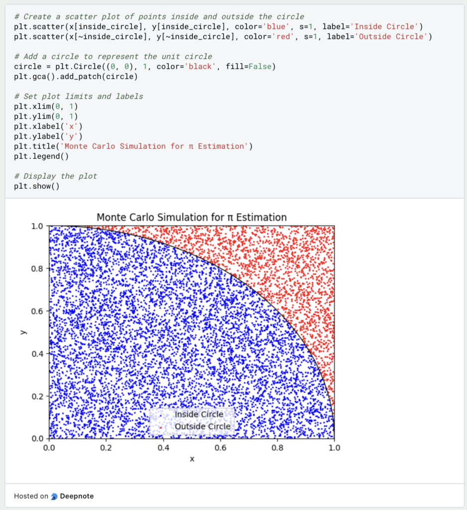
Step 6: Visualize the Results (Optional)

You can create a visual representation of the Monte Carlo simulation by plotting the points inside and outside the circle:

Step 7: Print the Estimation

Finally, print the estimated value of π::

By running this Python script, you can perform a Monte Carlo simulation to estimate the value of π. The more points you generate (larger num_points), the closer your estimation will be to the actual value of π. This example demonstrates a basic application of Monte Carlo methods, but they can be applied to a wide range of complex problems, including risk assessment, optimization, and more.

This is what you should take with you

• Monte Carlo methods are versatile and widely applicable for solving complex problems in various fields, from finance and engineering to physics and machine learning.
• They provide a powerful approach to estimating numerical results or probabilities through random sampling, making them invaluable for simulations and risk assessment.
• Monte Carlo simulations allow for the modeling of real-world scenarios by incorporating randomness and uncertainty into the analysis, resulting in more accurate predictions.
• Despite their reliance on randomness, Monte Carlo methods are computationally efficient and scalable, making them suitable for large-scale simulations and optimization tasks.
• These methods require careful consideration of sample size, convergence, and computational resources. They may also face challenges in high-dimensional spaces or when dealing with rare events.
• Monte Carlo techniques play a vital role in modern technologies, including finance for pricing derivatives, physics for simulating particle behavior, and machine learning for hyperparameter tuning and uncertainty quantification.
• As computational power continues to grow, Monte Carlo methods evolve with more sophisticated algorithms and applications, ensuring their relevance in solving complex problems.

Other Articles on the Topic of Monte Carlo Methods

The LMU University of Munich has interesting course slides about the topic that you can find here.