In the realm of statistics and data-driven decision-making, uncovering the parameters that best describe a given probability distribution is a pursuit fundamental to understanding underlying processes and making accurate predictions. Maximum Likelihood Estimation (MLE) stands as a cornerstone of statistical modeling, providing a powerful framework for achieving this very objective.

Imagine being able to discern the most probable values for parameters that govern the distribution of data—MLE allows precisely this, serving as a guiding beacon for statistical inferences. It’s a methodology that underpins countless applications, from finance to biology, guiding decision-makers in diverse fields.

In this article, we embark on a journey through the intricacies of Maximum Likelihood Estimation. We’ll unravel the core concepts, delve into their mathematical foundations, explore practical applications, and understand how this versatile tool empowers us to extract valuable insights from data. Let’s demystify MLE and discover its immense potential in the realm of statistical inference.

What are Probability Distributions?

Probability distributions are a fundamental concept in statistics and probability theory, serving as the cornerstone for understanding uncertain events and their likelihoods. A probability distribution describes the likelihood of various outcomes in a probabilistic event. It assigns probabilities to each possible outcome, indicating how likely each outcome is to occur. These probabilities follow certain rules, providing a structured way to quantify uncertainty.

In a discrete probability distribution, the possible outcomes are distinct and separate, such as the outcomes of rolling a die. On the other hand, a continuous probability distribution deals with outcomes that form a continuous range, like the heights of individuals in a population.

Key Concepts:

1. Probability Mass Function (PMF): The PMF defines the probabilities for each discrete outcome in a discrete probability distribution. It provides a complete profile of the distribution’s behavior.
2. Probability Density Function (PDF): In continuous probability distributions, the PDF represents the probabilities associated with different intervals. Unlike a PMF, a PDF doesn’t give the probability at a specific point but within a range.

Common Probability Distributions:

• Uniform Distribution: All outcomes have equal probabilities. For instance, when rolling a fair die, each face has a probability of 1/6.
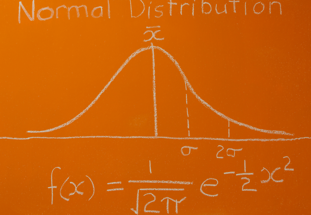
• Normal Distribution (Gaussian Distribution): A symmetric, bell-shaped distribution widely used in statistics. Many natural phenomena, such as heights or exam scores, follow this distribution.
• Binomial Distribution: Models the number of successes in a fixed number of independent Bernoulli trials, each with the same probability of success.
• Poisson Distribution: Describes the number of events occurring in a fixed interval of time or space, given a constant average rate of occurrence.
• Exponential Distribution: Models the time between events occurring in a Poisson process, where events occur continuously and independently at a constant average rate.

Understanding these probability distributions and their properties equips statisticians, data scientists, and researchers with powerful tools to analyze data, make predictions, and gain valuable insights into various phenomena. As we delve deeper into Maximum Likelihood Estimation, a firm grasp of probability distributions will prove instrumental in our exploration of statistical inference.

What is the Likelihood Function?

Understanding the likelihood function is essential to grasp one of the most powerful concepts in statistics – Maximum Likelihood Estimation. The likelihood function is a fundamental tool used to estimate the parameters of a statistical model, providing a bridge between observed data and the parameters that characterize the underlying probability distribution.

Definition and Core Idea:

The likelihood function, often denoted as \( \mathcal{L}(\theta \mid \mathbf{x}) \), quantifies the probability of observing the given data \( \mathbf{x} \) under a specific set of model parameters \( \theta \). In simpler terms, it answers the question: How probable is the observed data, assuming a particular configuration of model parameters?

The concept hinges on the fundamental principle of conditional probability. Given the parameters \( \theta \), the likelihood function treats the observed data \( \mathbf{x} \) as a function of these parameters. However, crucially, it treats the parameters \( \theta \) as variables and the data \( \mathbf{x} \) as fixed.

Mathematical Formulation:

For a set of observed data points assumed to be independently and identically distributed (an important assumption), the likelihood function is often expressed as the product of the probabilities associated with each data point:

\(\)\[\mathcal{L}(\theta \mid \mathbf{x}) = f(x_1 \mid \theta) \times f(x_2 \mid \theta) \times \ldots \times f(x_n \mid \theta) \]

where \( f(x_i \mid \theta) \) represents the probability density function (PDF) or probability mass function (PMF) of the statistical model associated with each data point.

Role in Maximum Likelihood Estimation:

The primary goal of Maximum Likelihood Estimation is to find the set of model parameters \( \theta \) that maximize the likelihood function \( \mathcal{L}(\theta \mid \mathbf{x}) \), given the observed data \( \mathbf{x} \). Mathematically, this is expressed as:

\(\) \[\hat{\theta}_{\text{MLE}} = \arg\max_{\theta} \mathcal{L}(\theta \mid \mathbf{x}) \]

In simpler terms, MLE seeks the parameter values that make the observed data the most probable, considering the assumed statistical model.

Understanding the likelihood function is foundational for statistical inference, enabling the estimation of parameters and facilitating insights into the behavior of various statistical models. As we explore Maximum Likelihood Estimation, a thorough grasp of the likelihood function will prove crucial to harness its full potential in statistical analysis and modeling.

What is the Log-Likelihood Function?

In statistical estimation, the log-likelihood function is a crucial tool that simplifies complex calculations and aids in the efficient estimation of model parameters. The log-likelihood function is the logarithm of the likelihood function, often used for numerical stability and mathematical convenience.

The key points of this function are:

1. Logarithmic Transformation: The log-likelihood function, denoted as \( \log(\mathcal{L}(\theta \mid \mathbf{x})) \), is obtained by taking the natural logarithm of the likelihood function. This transformation does not alter the optimization goal, as logarithmic functions preserve the location of maxima.
2. Advantages: Log-likelihood offers computational benefits, converting products (from the likelihood) into sums, simplifying mathematical operations and reducing the risk of numerical underflow.
3. Maximum Log-Likelihood: Similar to the likelihood function, the goal in Maximum Log-Likelihood Estimation (MLLE) is to find the set of model parameters \( \theta \) that maximize the log-likelihood function.
4. Statistical Estimation: Statisticians and data analysts often prefer working with log-likelihood due to its ease of use, particularly in cases involving large datasets and complex models.

By understanding the log-likelihood function and its significance, practitioners can navigate statistical analysis and parameter estimation more efficiently, aiding in the pursuit of accurate models and insightful conclusions.

What is the MLE procedure?

Maximum Likelihood Estimation is a fundamental method used in statistics and machine learning to estimate the parameters of a statistical model. The procedure seeks to find the values of these parameters that maximize the likelihood function, which measures the likelihood of observed data given the model.

Here’s an outline of the MLE procedure:

1. Formulate the Likelihood Function: Begin by defining the likelihood function \( L(\theta \mid x) \), which represents the probability of observing the given data (x) given the parameters \( \theta \) of the model.
2. Take the Logarithm: To simplify calculations, often the logarithm of the likelihood function, called the log-likelihood function, \( \log L(\theta \mid x) \), is used. This step does not alter the location of the maximum, as the logarithm is a monotonically increasing function.
3. Derive the Score Function: Compute the score function (also known as the gradient of the log-likelihood function) with respect to the parameters. The score function provides the direction of steepest ascent, pointing towards the maximum likelihood estimate.
4. Set the Score Function to Zero: Equate the score function to zero to find the critical points. Solving this equation yields the values of the parameters that maximize the log-likelihood.
5. Check Second Derivatives: Confirm that the critical points found are indeed maxima by examining the second derivatives of the log-likelihood. The Hessian matrix (matrix of second partial derivatives) should be negative definite at the maximum point.
6. Estimate Parameters: The values obtained by solving the system of equations from the score function represent the maximum likelihood estimates of the parameters \( \hat{\theta} \).

The maximum likelihood estimates \( \hat{\theta} \) are considered the most probable values for the parameters, given the observed data. MLE is widely used due to its desirable statistical properties, such as consistency, asymptotic normality, and efficiency.

In summary, the maximum likelihood estimation procedure aims to find the parameter values that make the observed data the most probable under a specified statistical model, making it a powerful tool in statistical inference and machine learning.

What are the properties of MLE?

Maximum Likelihood Estimation is a powerful statistical method used to estimate parameters of a probability distribution based on observed data. MLE possesses several desirable properties that make it a widely utilized tool in various fields of statistics and machine learning. Here are some key properties of MLE:

1. Consistency: As the sample size increases, MLE converges in probability to the true values of the parameters being estimated. In simpler terms, as you collect more data, these estimates approach the actual, population-level parameter values.
2. Asymptotic Normality: For a large enough sample size, the MLE estimates have an approximate normal distribution with a mean equal to the true parameter values and a variance that decreases with the sample size. This property is fundamental for constructing confidence intervals and hypothesis tests.
3. Efficiency: Among the class of consistent estimators, MLE is often the most efficient, providing the smallest possible variance. In statistical terms, MLE achieves the Cramér-Rao lower bound, ensuring the highest precision in estimating the parameters.
4. Invariance: MLE is invariant under transformations. If \( \hat{\theta} \) is the MLE for a parameter \( \theta \), then any function \( g(\hat{\theta}) \) is the MLE for \(g(\theta) \). This property is valuable when estimating derived quantities or functions of the parameters.
5. Sufficiency: MLE often leads to sufficient statistics, i.e., summary statistics that contain all the information about the parameters. This property helps in reducing the dimensionality of the data while retaining essential information for estimation.
6. Bias and Efficiency Trade-off: This estimation method tends to be asymptotically unbiased, meaning that as the sample size grows, the bias of the estimate diminishes. However, MLE can be biased for small sample sizes. The bias-efficiency trade-off implies that the method often sacrifices bias for efficiency.
7. Robustness: MLE is known to be asymptotically robust, meaning that it remains consistent even when the underlying assumptions of the probability distribution are slightly violated. This makes MLE a resilient estimation method in real-world scenarios where assumptions may not hold perfectly.

Understanding these properties is crucial for practitioners to effectively utilize MLE in a wide range of statistical applications. These properties affirm the reliability, accuracy, and robustness of MLE, making it a cornerstone of modern statistical estimation.

What are the advantages and disadvantages of MLE?

Maximum Likelihood Estimation is a widely used statistical method for estimating parameters of a probability distribution based on observed data. Like any statistical technique, MLE comes with its set of advantages and disadvantages, which are essential to consider when applying it to real-world problems.

One significant advantage of MLE is its efficiency and asymptotic properties. Among a class of consistent estimators, MLE provides the most efficient estimates, achieving high precision and accuracy as the sample size increases. Furthermore, MLE estimators are consistent, meaning they converge to the true parameter values with an increasing amount of data, ensuring accuracy in estimation.

Another advantage is the invariance of MLE under various transformations. This flexibility allows for the estimation of a wide range of models, making MLE highly adaptable. Additionally, MLE is asymptotically robust, retaining consistency even when underlying distribution assumptions are slightly violated, a valuable feature for real-world scenarios where assumptions may not perfectly hold.

However, MLE is not without its drawbacks. It can be sensitive to outliers or anomalies in the data, potentially leading to biased or inaccurate estimates, especially in small sample sizes. Additionally, the assumption of a specific probability distribution for the data is a limitation, and if this assumption is significantly incorrect, the estimates can be unreliable. For small sample sizes, MLE can be biased, impacting the accuracy of the estimates, and in multivariate problems with numerous parameters, MLE becomes computationally complex. Lastly, MLE’s performance can be highly dependent on the initial values chosen for the optimization process, which may lead to different local optima and affect the accuracy and stability of the estimates.

Understanding these advantages and disadvantages is crucial for researchers and practitioners in making informed decisions about when and how to utilize MLE effectively. Consideration of the specific characteristics of the data and the problem at hand is key to maximizing the benefits of MLE while mitigating its limitations.

How does MLE compare to other estimation methods?

In the realm of statistical parameter estimation, several methods compete for prominence, each with its own strengths and weaknesses. Maximum Likelihood Estimation stands out as a popular and widely utilized technique, but how does it compare to other estimation methods?

One of the significant differences lies in the underlying philosophy. MLE strives to find the parameter values that maximize the likelihood function given the observed data. This is in contrast to other methods like Method of Moments (MoM) or Least Squares Estimation (LSE), which focus on matching sample moments or minimizing the sum of squared differences, respectively.

In terms of efficiency and statistical properties, MLE often outshines other methods. Its estimators are asymptotically efficient, achieving the smallest possible variance as the sample size grows, assuming certain regularity conditions. This efficiency property positions the algorithm as a preferred choice when precision and accuracy are paramount.

However, MLE’s efficiency advantage may come at a cost, particularly when compared to simpler methods like MoM. MLE requires solving complex optimization problems, which can be computationally intensive and sensitive to the choice of initial values. MoM, on the other hand, tends to be computationally straightforward and less prone to convergence issues.

When assumptions about the underlying distribution are accurate, MLE performs exceptionally well. Yet, it can be highly sensitive to distributional assumptions, and if these assumptions are violated, the estimates may be biased or inconsistent. In contrast, methods like LSE are robust and more forgiving in the face of distributional misspecifications.

In practice, the choice of estimation method often depends on the specific problem, data characteristics, and computational considerations. Researchers and practitioners weigh the trade-offs between accuracy, computational complexity, and robustness against distributional assumptions when selecting an appropriate estimation method.

In conclusion, MLE is a powerful and widely favored estimation method due to its efficiency and desirable asymptotic properties. However, its reliance on accurate distributional assumptions and computational complexity may lead practitioners to opt for alternative methods like MoM or LSE based on the specifics of the problem at hand. Understanding these trade-offs is essential for selecting the most suitable estimation technique for a given scenario.

This is what you should take with you

• MLE is a highly efficient estimation method, achieving the smallest possible variance for large sample sizes, assuming regularity conditions are met.
• It heavily relies on accurate distributional assumptions. If these assumptions are incorrect, the estimates can be biased or inconsistent.
• The estimation method involves solving complex optimization problems, which can be computationally intensive and sensitive to initial values. This complexity increases with the dimensionality of the parameter space.
• MLE is widely applicable across various domains, from finance to biology, due to its flexibility in modeling diverse types of data and parameters.
• The Maximum Likelihood Estimation is particularly advantageous for large samples where its efficiency properties shine, making it a preferred choice in such scenarios.
• Practitioners must carefully consider the trade-offs between computational complexity, robustness against assumptions, and the desire for efficient estimates when choosing MLE over alternative estimation methods.
• Despite its challenges, MLE remains a versatile and powerful tool in statistics, playing a central role in various statistical modeling and inference procedures.

Other Articles on the Topic of the Maximum Likelihood Estimation

Here you can find an article about how to do the Maximum Likelihood Estimation in Python.