The median plays a central role in statistics and data analysis, as it can be used as a measure of the central tendency of a data set. It is the value in the data set that forms the center and divides the numbers into two equal parts. Compared to the mean value, it is not susceptible to outliers and provides a reliable picture of the central situation even with unevenly distributed data. Due to this property, the ratio is used in various fields, such as medicine, social sciences or economics.

In this article, we explain all the details about the median and go into detail about the calculation of this key figure using various examples. We also compare it with other statistical indicators such as the mean or the mode and show which applications use it. A complete picture also includes explaining the advantages and disadvantages of this key figure in detail so that you can make an informed decision as to whether its use is justified. Finally, we look at how to calculate the ratio in Python or Excel.

What is the Median?

The median is a statistical key figure that provides a statement about the central tendency of the data set. It is the value that lies exactly in the middle of an ordered data series so that all elements in one half of the data set are smaller than the median and all elements in the other half of the data set are correspondingly larger.

This property makes it a robust choice, as it remains identical even with unevenly distributed data. The median does not change if the specific values of the lower half change, as long as the number of values remains the same and they are all still smaller than the median value. This means that even extreme outliers do not have a major impact for the time being.

The mean value, on the other hand, calculates the arithmetic average of the data set instead of finding the middle of the data set. This means that data points with extremely large or small values have a strong influence on the average. The median is used in a wide variety of applications where outliers may occur to obtain a more realistic assessment of the central situation. In income surveys, for example, the two key figures sometimes differ very significantly.

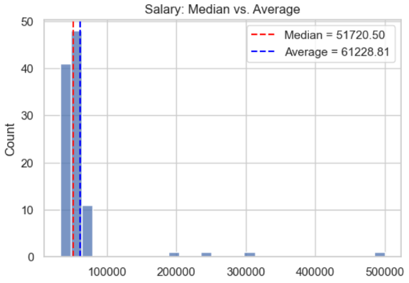
This diagram shows the salaries of more than one hundred people. It can be seen that the majority of the respondents, around fifty people, have an annual salary of around $50,000. However, there are also a few outliers of employees with a much higher salary of $200,000 up to $500,000. The average reacts much more strongly to these people and gives the average salary as around $60,000, while the median is more robust to the outliers and correctly recognizes that the majority of people earn less than $60,000.

How is the Median calculated?

The median is the middle value in a data series and, depending on the size of the data series, can be a value from the set or a value that does not occur directly in the set. In the first step of the calculation, the data series is sorted in ascending order of size. Once this has been done, the further calculation depends on whether the number of elements is even or odd.

Data Sets with an odd Number of Elements

If there is an odd number of elements in the data series, calculating the median is much easier. To do this, simply take the value from the sorted data series that lies exactly in the middle. The fact that the number is odd also ensures that such a value exists.

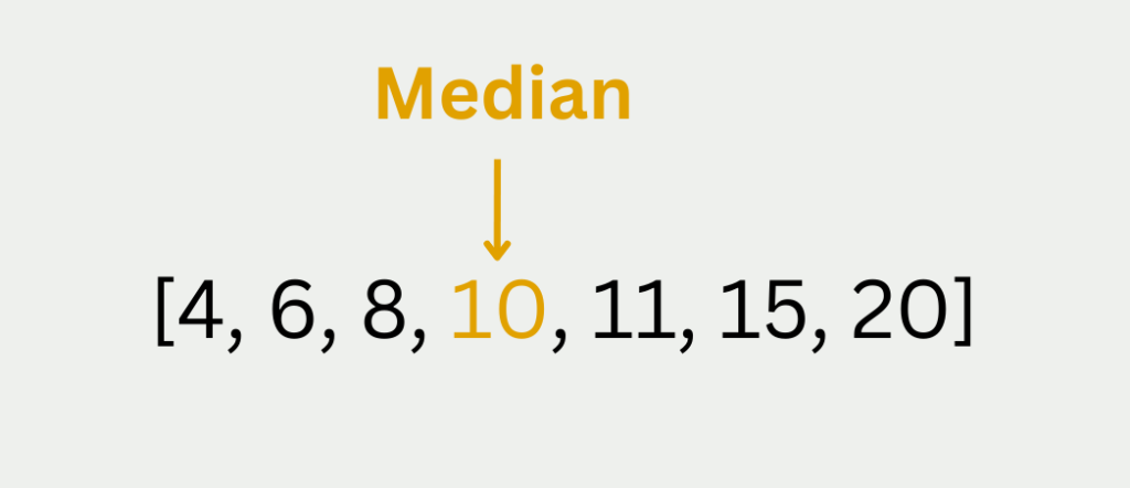
In the data series [3,7,9], for example, the 7 is exactly in the middle, as there is exactly one value that is larger and exactly one smaller value. The median of this data series is therefore 7. The data series [3,7,9,13,18] has five elements and therefore also an odd size. In this case, the 9 lies exactly in the middle of the data series and therefore the result is 9.

Data Sets with an even Number of Elements

With an even number of elements, the approach just described cannot be used because no data point lies exactly in the middle of the data series. In the data series [3,7,9,11], for example, this center point does not exist. Therefore, you have to make do by using the two middle values, in this case, 7 and 9, and calculating the average, i.e. (7+9)/2 = 8. The median in this data series is therefore 8.

This procedure makes it clear why the median is robust against outliers, as the values outside the middle are not relevant for the calculation as long as they do not change the order of the individual elements. For example, if we use the series [3,7,9], 7 remains the median, even if the value of the other two elements changes significantly. This means that 7 is also the center of the data series [1,7,100] and it is also the median of the data series [0.001,7,10000].

These two cases can be summarized using the following formula:

\(\)\[
\text{Median} =
\begin{cases}
x_{\frac{n+1}{2}}, & \text{if } n \text{ is odd} \\[10pt]
\frac{x_{\frac{n}{2}} + x_{\frac{n}{2} + 1}}{2}, & \text{if } n \text{ is even}
\end{cases}
\]

What are Median, Mode, and Mean and how do they differ?

The median, mode and mean are different measures that describe different aspects of the “middle” of a data set. Depending on the type and characteristics of the data, each of these measures has its advantages and disadvantages, which we examine in more detail in this section. A central aspect for the selection of the appropriate measure is also the distribution of the data, which includes, for example, whether outliers are present.

Mean Value

The mean value is calculated by adding up all the data points in a data set and then dividing them by the number of data points. It thus serves as a kind of balance point for the data set. However, this calculation also makes the mean value susceptible to outliers, i.e. particularly high or low values, and to uneven distributions. In these cases, the mean value may not provide an accurate picture of the data set.

Since the mean value includes all values with equal weight in the calculation, a single extremely high or low value can strongly influence the average. Such a value can therefore result in the midpoint no longer representing the typical center of the data set. This makes the mean value unsuitable for asymmetrical or distorted data.

Example: Suppose we have a data set on the distribution of income in a small group. The following incomes are determined: [30.000, 32.000, 35.000, 500.000]. From looking at the data, we would assume purely by feeling that an “average person” in this data set earns approximately between 32,000 and 35,000. However, due to the very strong outlier, we get a calculated average of (30,000 + 32,000 + 35,000 + 500,000) / 4 = 149,250. However, this value is much higher than the typical incomes we observe in the dataset, which can be attributed to the highest income of 500,000.

Due to these properties, the mean value is particularly suitable for normally distributed data without extreme outliers, such as those found in chemistry, physics, or financial analysis. These can often fall back on a uniform distribution of data.

Median

The median is the middle value of a data series and divides the data set so that half of the data lies above and the other half below it. This characteristic makes this key figure significantly less sensitive to outliers or strongly deviating data points, as only the position of the extreme data points plays a role and not their absolute value.

For the income example above, this means that the median must lie exactly between 32,000 and 35,000, as this is the middle of the data set. This results in a value of (32,000 + 35,000) / 2 = 33,500, which provides a more realistic statement about the middle of the data distribution compared to the mean value, as it is not distorted by the outlier income.

Due to this property, the median is primarily used in applications in which data is often distorted and outliers play a major role, such as in income statistics, real estate prices, or medical data.

Mode

The mode differs from the two key figures presented so far and describes the most frequent value in a data series. It is therefore a measure of central tendency that deals exclusively with the frequency of values. This property means that the mode is the only one that can also be used for nominal data, i.e. data that is not numerical.

The mode is often used in surveys and market research, as it offers the possibility of identifying the most frequent answers or popular products. However, this also highlights the main problem with the mode, namely when a series is ambiguous so that two values occur the same in the survey. For example, if both “Audi” and “BMW” are mentioned equally frequently in a survey of the most popular car brands, then the data series is said to be bimodal, as exactly two categories occur most frequently. In a multimodal data series, there are even more than two values that were mentioned most frequently in the survey.

Overall, the following chart offers a good opportunity to make a quick decision in favor of one of the key figures:

Compared to the mean and the mode, the median offers a balanced way of numerically expressing the central tendency of a data set. It is particularly strong in the case of distorted data with outliers, as it cannot be influenced by these as long as the mean value of the data set remains the same. The mean value, on the other hand, is more suitable for normally distributed data without the risk of outliers and the mode can also be used for nominal data sets.

What are the Advantages and Disadvantages of the Median?

The median is a frequently used measure to determine the central tendency of a data set. In this article, we have already mentioned some of the advantages and disadvantages of using this key figure. In this section, we want to summarize the points again and also include a few new aspects.

Advantages

• Robustness against outliers: As already explained several times, the main advantage of the median is that it changes little or not at all even in the case of extreme values and outliers, and, in contrast to the mean value, is significantly more robust against these phenomena. As it relates solely to the position of the data, the level of the data and its differences only play a subordinate role.
• Better representation with skewed distributions: For skewed distributions, such as income statistics or real estate prices, the median often represents a more realistic picture compared to the mean. Such data is often skewed to the right, which causes the mean to be pulled upwards unnaturally and thus a better center of the data can be displayed.
• Transformation invariant: Although the median is a non-linear scale, it is not changed by monotonic transformations. Linear transformations, such as the multiplication of all data set values by a fixed constant or the addition of a fixed value, change the mean value directly. However, the order of the data set remains the same, so the value does not change. For example, the data set can be logarithmized and the new value then simply corresponds to the logarithm of the old median.
• Easy interpretation: This key figure can be interpreted quickly and easily, even with large data sets, and can therefore be easily understood by a non-specialist audience. The way it is calculated makes it much less complicated, which makes it more acceptable to the audience in reports or presentations, for example.
• Use with ordinal data: Finally, unlike the average, the median can also be used with ordinal data with rating scales or rankings, making it much more flexible to use. In market research, for example, this is a further advantage that makes it possible for the data to be neither measurable nor interval-scaled.

Disadvantages

• Loss of detail: As the median is only based on the location of the data and does not take into account the distances between the data points, this key figure loses important information about the location and distribution of the data. This is an exclusion criterion in distributions in which the distances play an important role, such as for measured values in scientific experiments.
• Sensitivity to data changes in even data sets: For even data sets, the median is calculated as the average of the two middle data points. This can make it susceptible to data changes in such a scenario, especially if the sample is particularly small.
• Limited significance with normally distributed data: With normally distributed or symmetrical data, the median hardly differs from the mean, as outliers only play a minor role. As both values are then almost identical, the median offers no advantages and may even provide less information about the distribution itself. The mean, on the other hand, together with the standard deviation, can already describe important properties of the distribution.
• Lack of applicability in statistical tests: Many statistical tests, such as the t-test or the analysis of variance, rely on the mean as a measure of the central tendency. The median is often not applicable here and would first have to be transformed at great expense to be applicable for these inferential statistical tests.
• Not suitable for all types of data: Although the median can be of great use in many applications, in individual cases it may only have limited informative value. For example, in multimodal distributions, where the data has multiple clusters of values, the median does not necessarily represent the central point that accounts for all clusters equally.

Just like other statistical indicators, the median has advantages and disadvantages that should be weighed up before use. The main advantages are that it does not react as strongly to outliers as the mean value and can therefore provide a better picture of the central tendency. In normally distributed data distributions, however, it hardly differs from the mean value and information on the distances between the data points is still lost.

What Challenges does the Median pose and how can they be solved?

Especially when working with large amounts of data and in special data contexts, working with the median can pose challenges. In this section, we look at some scenarios and how to deal with them effectively.

Efficiency with large Amounts of Data

The median is based on the fact that a list of values must first be sorted and then the middle element from this list is selected. With very large amounts of data, this task can be very computationally intensive and take a lot of time. To ensure that the median can still be calculated efficiently, the so-called QuickSelect algorithm is used, which offers an efficient method for finding the \(k\)-smallest element in an unsorted list. This saves sorting the list, which takes \(O(nlogn)\) time on average. The QuickSelect algorithm, on the other hand, works with the average linear time (\(O(n)\)).

For this purpose, any element, the so-called pivot element, is selected from the list. Similar to QuickSort, the list is then partitioned around this element so that all elements that are smaller than the pivot are moved to the left partition, and all elements that are larger than the pivot are moved to the right partition. This partitioning tells you how many elements are smaller than the pivot.

Assuming \(m\) is the number of elements in the left partition, the following three cases result:

• \(k = m+1\): There are exactly \(k-1\) elements in the left partition. This means that the median has already been selected as the pivot.
• \(k \leq m\): The median we are looking for is therefore in the left-hand partition, as there are more than \(k\) values in the left-hand partition and therefore there are also values in the left-hand partition that are even greater than \(k\). The algorithm can therefore be applied recursively to the left partition.
• \(k \geq m+1\): In this case, there are fewer than \(k\) values in the left-hand partition, so the value you are looking for must be in the right-hand partition. The algorithm is therefore applied recursively to the right-hand partition.

This procedure significantly reduces the time required for the calculation and data sets with different sizes can be processed efficiently.

Median in grouped Frequency Distributions

In grouped data sets, the individual values of the data set are not available, but only the grouped frequency distributions are given, i.e. the number of values in a class. A common example is the evaluation of school grades, where the individual grades are not known, but only how many students have achieved grades between 1 and 2. This makes it difficult to determine the median.

To solve this problem, the cumulative frequency is calculated for each grade by successively adding up the frequencies of the grades. The number of total observations, i.e. the size of the data set, and dividing this by two. The median is then in the group in which the cumulative frequency exceeds this threshold for the first time.

Median with weighted Data

In weighted data sets, the individual data points are given different weightings to prevent distortion in the data set. For example, if you want to survey all age groups, but could only interview very few older people due to the survey method, then the few senior citizens who could be interviewed are given a higher weighting in the data set so that there is no bias towards the younger respondents. The weighted median must then be determined accordingly for such a data set.

This is determined in such a way that around 50 % of the total weights are below and around 50 % of the total weights are above. Depending on the data set, it may not be possible to find the exact center. This approximation must therefore be used.

By using these methods, the median can also be applied to special data sets that are grouped, weighted, or simply very large.

How can you calculate the median in Python, Excel, and other programs?

Calculating the median is an important step in many statistical analyses and can be done quickly and easily using Python or Excel. In this section, we take a closer look at the calculation using simple examples.

Calculating the Median in Excel

In Excel, the median can be calculated easily using a function. For example, you can collect the incomes in a data set in a column and apply the function in a new cell by defining the range in which the figures are stored.

In our case, we have stored ten income data in column A and overwritten it with the heading “Incomes”. Accordingly, the numerical values are stored in cells A2 to A11.

The median can now be calculated in a new cell by calling the function.

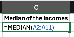
In the round brackets, we define the number range in which the income is stored and receive the final result after pressing the ENTER key.

With the help of these simple steps, the key figure for a data series can be calculated quickly in Excel.

Calculating the Median in Python

In Python, you can use various libraries to calculate the median, such as NumPy or Pandas. In NumPy, you store the data in a list and then use the corresponding function to which the list is then passed.

The use of NumPy can be particularly efficient with large amounts of data, as the calculation has been specially optimized. However, if the data is stored in a DataFrame, the use of Pandas is the obvious choice. This library already provides a function that can be applied directly to a DataFrame column.

Median Calculation in R

This key figure can be used directly in R without having to import a library. The values of the data set are simply stored in a vector. The key figure can then be determined using this function.

data <- c(3, 7, 2, 9, 5)

median_value <- median(data)

print(median_value)

If there are missing values in the data set, the calculation can be adjusted using an additional parameter. If this is not done, the normal function would return NA. The solution for this situation is the argument na.rm = TRUE, so that the missing values are simply skipped in the calculation:

data_with_na <- c(4, 7, NA, 10, 6, NA, 9) 

median_na <-median(data_with_na, na.rm = TRUE) 

print(median_na)

Median Calculation in SQL

There is no direct function in SQL that can be used to calculate the median of a column. A simple alternative would therefore be to load the data set into a DataFrame using pandas and continue the calculation there. If this is not an option and you have to stay in SQL, you can determine the median indirectly by selecting the middle value from an ordered list.

Let’s assume we have a simple table sales of a company and in it the column amount in which the quantity sold is stored. Using the following query, we can output the corresponding row in the table containing the median for a data set with an odd value.

WITH ordered AS (

    SELECT amount, 

           ROW_NUMBER() OVER (ORDER BY amount) AS row_num,

           COUNT(*) OVER () AS total_rows

    FROM sales

)

SELECT amount AS median

FROM ordered

WHERE row_num = (total_rows + 1) / 2;

These are:

• ROW NUMBER() OVER (ORDER BY amount) AS row_num: This expression numbers the rows of the data set that were previously sorted in ascending order by amount.
• COUNT(*) OVER () AS total_rows: In this section, the size of the data set is stored in the variable total_rows.
• The WHERE clause ensures that if the size of the data set is odd, exactly the middle element is used. Assuming we have a data set size of 5, the WHERE clause filters the rows with the number (5+1)/2 = 3.

With an even data set size, however, the query must be modified slightly so that the mean value of the two middle elements is calculated. This results in a new WHERE clause:

WITH ordered AS (

    SELECT amount, 

           ROW_NUMBER() OVER (ORDER BY amount) AS row_num,

           COUNT(*) OVER () AS total_rows

    FROM sales

)

SELECT AVG(amount) AS median

FROM ordered

WHERE row_num = (total_rows) / 2 

   OR row_num = (total_rows + 1) / 2;

As we have seen, the median calculation is possible in various software systems. However, when working with larger data sets, programming languages such as R or Python should be used for the sake of simplicity. These then also offer the option of further data analysis steps being possible directly.

Which Applications Use the Median?

The median is a central position parameter in statistics that is used in many applications and is particularly useful when data is asymmetrically distributed or contains outliers. However, there are also many other areas of application outside of statistics:

• Economics & Finance: For the realistic representation of wages, rents, or prices, the median is essential to be able to make a reliable statement about the middle. For example, the median rent in a city paints a realistic picture of citizens’ housing costs without being distorted by very cheap or very expensive apartments.
• Machine Learning: In image processing in particular, the median is used as a filter to reduce noise to skillfully replace sudden and erroneous pixels. Data sets can also be processed using this key figure to compensate for incorrect values and replace them with a mean value for this attribute.
• Medicine & Biostatistics: In the field of hospital planning, it makes sense to calculate the median length of stay of patients to be able to plan and ensure the logistics behind it, such as staff, hospital rooms, or catering, accordingly. In an average analysis, on the other hand, these figures could be set too low or too high due to outliers.
• Social Sciences: In the social sciences, the median is used in demographic research to determine the median age of the population, for example.

The median as a key figure has become indispensable in many areas of analysis and is mainly used to reduce the influence of outliers. It plays a central role in the fields of economics, machine learning, medicine, and social sciences in particular.

What Extensions of the Median are there?

The median is already a very simple position parameter that can be used in a wide variety of applications. However, there are special cases in which the classic median is not sufficient, which is why individual extensions must be used. In this section, we briefly present some of the most important extensions.

Moving Median for Time Series Analysis

In time series analysis, so-called moving averages are often considered, i.e. the average of a past period, such as the last five days or three months. However, extreme values in these periods can be heavily distorted, which is why the moving median can also be used, which is more robust in this respect. The value for the current day is then simply calculated by using the values from a previous period and calculating the median using the familiar definition.

The moving median is used, for example, in the valuation of share prices to identify a general trend that is not too strongly influenced by outliers. In medicine, on the other hand, it helps with heart rate sensors, as these can be subject to short-term measurement errors or disturbances. By using the moving median, the actual signal can be filtered out and analyzed.

Multidimensional Median for Vector Data

So far we have only looked at the median in one dimension. However, there are various applications, such as image processing or machine learning in general, which work with multidimensional data that is available in vectors. The multidimensional median is then used for this, which calculates the one-dimensional median in each dimension and then creates a corresponding vector from the values.

In image processing, this procedure can be helpful removing random noise from images and is therefore used as a so-called median filter in the pre-processing of images. This is where so-called impulse noise can occur if digital images contain random light and dark pixels due to damage. This filter is then used to replace the damaged pixels with the center of the surrounding pixels.

In machine learning, the multidimensional median is also used in k-means clustering, for example. This algorithm aims to assign the elements of a data set to different clusters. For this purpose, different cluster assignments are tested iteratively and a cluster center is formed in each step, which represents the middle of a cluster. The multidimensional median is then used for this calculation.

Geographical Median for the Location Analysis

The geographical median describes the point that has the shortest total distance to all other points in the data set. For this purpose, the distance to all other points is calculated and added up for each point and then the element with the shortest total is selected.

This procedure is used in business planning, for example, when different locations for a logistics center are evaluated or when a new hospital location is to be determined. It can also be used in network analysis to find the optimal location for a new mobile phone mast.

These extensions make the median a flexible and powerful tool that can be used in many standardized applications and can also be customized for more specific data analyses.

This is what you should take with you

• The median is a basic key figure that provides a statement about the central tendency of the data set.
• It determines a value that is exactly in the middle of the data series and is therefore not so strongly influenced by outliers compared to the mean value.
• In addition to the median, the mean value or the mode can also be used to determine the central tendency of a data set.
• The median also has disadvantages, such as the fact that information about the distances between the data points is lost.
• Various computer programs can be used to calculate this key figure, such as the Python programming language or Excel.

Other Articles on the Topic of Median

This link will get you to my Deepnote App where you can find all the code that I used in this article and can run it yourself.