The gradient descent method is a solution guide for optimization problems with the help of which one can find the minimum or maximum of a function. This method is used in the field of Machine Learning for training models and is known there as the gradient descent method.

What is the Gradient Descent Method used for?

The goal of artificial intelligence is generally to create an algorithm that can make a prediction as accurately as possible with the help of input values, i.e. that comes very close to the actual result. The difference between the prediction and the reality is converted into a mathematical value by the so-called loss function. The gradient descent method is used to find the minimum of the loss function because then the optimal training condition of the model is found.

The training of the AI algorithm then serves to minimize the loss function as much as possible in order to have a good prediction quality. The Artificial Neural Network, for example, changes the weighting of the individual neurons in each training step to approximate the actual value. In order to be able to specifically address the minimization problem of the loss function and not randomly change the values of the individual weights, special optimization methods are used. In the field of artificial intelligence, the so-called gradient descent method is most frequently used. 

Why do we approach the Minimum and not just calculate it? 

From calculus, we know that we can determine a minimum or maximum by setting the first derivative equal to zero and then checking whether the second derivative is not equal to 0 at this point. Theoretically, we could also apply this procedure to the Artificial Neural Network loss function and use it to accurately calculate the minimum. However, in higher mathematical dimensions with many variables, the exact calculation is very costly and would take a lot of computing time and, most importantly, resources. In a neural network, we can quickly have several million neurons and thus correspondingly several million variables in the function. 

Therefore, we use approximation methods to be able to approach the minimum quickly and be sure after some repetitions to have found a point close to the minimum.

What is the basic idea of the Gradient Descent?

Behind the gradient descent method is a mathematical principle that states that the gradient of a function (the derivative of a function with more than one independent variable) points in the direction in which the function rises the most. Correspondingly, the opposite is also true, i.e. that the function falls off most sharply in the opposite direction of the gradient. 

In the gradient descent method, we try to find the minimum of the function as quickly as possible. In the case of artificial intelligence, we are looking for the minimum of the loss function and we want to get close to it very quickly. So if we go in the negative direction of the gradient, we know that the function is descending the most and therefore we are also getting closer to the minimum the fastest.

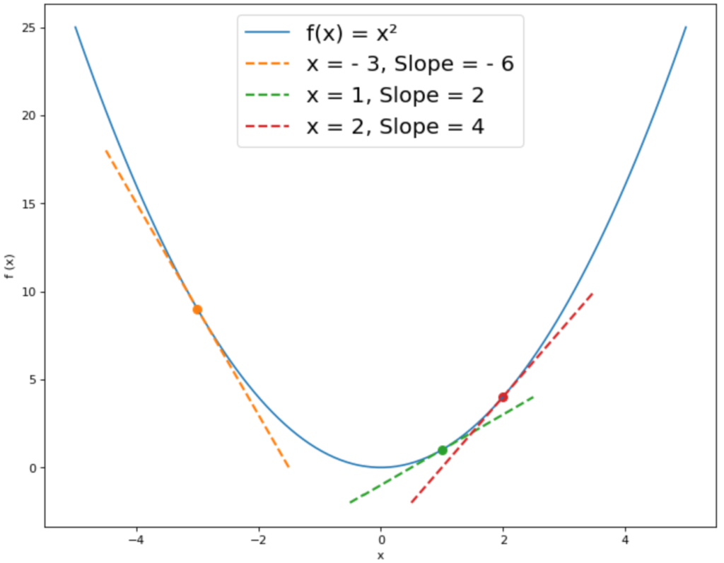
For the function f(x) = x² we have drawn the tangents with the gradient f'(x) at some points. In this example, the minimum is at the point x = 0. At the point x = -3, the tangent has a slope of -6. According to the gradient method, we should move in the negative direction of the gradient to get closer to the minimum, so – (- 6) = 6. This means that the x-value of the minimum is greater than -3.

At the point x = 1, however, the derivative f'(1) has a value of 2. The opposite direction of the gradient would therefore be -2, which means that the x-value of the minimum is less than x = 1. This brings us gradually closer to the minimum. 

In short, the gradient descent states:

• If the derivative of the function is negative at the point x, we go forward in the x-direction to find the minimum. 
• If the derivative of the function is positive at the point x, we go backward in the x-direction to find the minimum. 

In the case of a function with more than one variable, we then consider not only the derivative but the gradient. In multidimensional space, the gradient is the equivalent of the derivative in two-dimensional space. 

What do we need the Learning Rate for?

The gradient descent method gives us the corresponding direction for each starting point. However, it does not tell us how far we should go in the corresponding direction. In our example, we cannot know with the help of the gradient method whether we should go one, two, or even three steps in the positive x-direction at the position x = -3. 

With the help of the learning rate, we can set how large each step should be. There are approaches in which the value of the learning rate can change in each step, but in most cases, it is constant and is, for example, a value of 0.001. 

How do we find the optimal Learning Rate?

The decision for the size of the learning rate actually seems simple. With a small learning rate, we approach the minimum only very slowly, especially if our starting point is far away from the extreme point. On the other hand, if we use a larger learning rate, we may move faster toward the minimum, so we should pick a large learning rate. Unfortunately, it is not that simple.

For example, it may be the case that the starting point is already very close to the minimum without us knowing about it. Then a large learning rate may be too large so that we never arrive at the minimum. If we start with the function f(x) = x² at the point x=1 and use a learning rate > 1, we will not be able to arrive at the minimum x = 0 very quickly, because the distance to the minimum is only 1.

Thus, the choice of an appropriate learning rate is not very easy to answer and there is no optimal value that we can use. In Machine Learning, there is a name for such parameters: Hyperparameters. These are parameters within the model whose value is crucial for success or failure. This means it can happen that a poorly performing model becomes significantly better by changing a hyperparameter and vice versa. The learning rate is one of many hyperparameters and should simply be varied in different training runs until the optimal value for the model is reached.

What are the Problems with Gradient Descent?

There are two major problem areas that we may have to deal with when using the gradient method:

• We end up with a local minimum of the function instead of a global one: Functions with many variables very likely do not have only one minimum. If a function has several extreme values, such as minima, we speak of the global minimum for the minimum with the lowest function value. The other minima are so-called local minima. The gradient descent does not automatically save us from finding a local minimum instead of the global one. However, to avoid this problem we can test many different starting points to see if they all converge toward the same minimum. 

• Another problem can occur when we use the gradient descent method in the context of neural networks and their loss function. In special cases, e.g. when using feedforward networks, the gradient may be unstable, i.e. it may become either very large or very small and tend towards 0. With the help of other activation functions of the neurons or certain initial values of the weights, one can prevent these effects. However, this is beyond the scope of this article. 

How do we calculate the Gradient Descent in the Multidimensional Space?

For our initial example f(x) = x² the extreme point was very easy to calculate and also determinable without the gradient method. With more than one variable this is not so easy anymore. For example, let’s take the function f(x,y) = x² + y² and try to approach the minimum in a few steps.

1. Determination of the Starting Point: If we want to use the gradient descent method, we need a starting point. There are many methods to find an optimal starting point, but that is not what this article is about in detail. We simply start our search at point P(2,1).

2. Calculate the Derivative / Gradient: Next we have to calculate the first derivative of the function. In multidimensional space, this is called a gradient. It is the vector of all derivatives of the variables. In our case, the function consists of two variables, so we need to form two derivatives. One is the first derivative with x as a variable and the other is the first derivative with y as a variable:

\(\) \[f_x(x,y) = 2x \\ f_y(x,y) = 2y \]

The gradient is then simply the vector with the derivative with respect to x as the first entry and the derivative with respect to y as the second entry:

\(\) \[\nabla f(x,y) = \begin{bmatrix}
2x \\
2y \end{bmatrix} \]

3. Inserting the Starting Point: Now we insert our starting point into the gradient:

\(\) \[\nabla f(2,1) = \begin{bmatrix}
2*2 \\
2*1 \end{bmatrix} =
\begin{bmatrix}
4 \\
2 \end{bmatrix}
\]

4. Add Negative Gradient with Step Size to the Start Point: In the last step, we now go in the negative direction of the gradient from our starting point. That is, we subtract the gradient multiplied by the learning rate from our starting point. With a learning rate of 0.01 this means:

\(\) \[ P_2(x,y) = \begin{bmatrix}
2 \\
1 \end{bmatrix} – 0,01 *
\begin{bmatrix}
4 \\
2 \end{bmatrix} =
\begin{bmatrix}
1,96 \\
0,98 \end{bmatrix}
\]

Thus, we now have our new point P₂(1.96; 0.98) with which we can start the procedure all over again to get closer to the minimum.

This is what you should take with you

• The gradient descent is used to approach the minimum of a function as fast as possible.
• For this purpose, one iteratively goes at one point always in the negative direction of the gradient. The step size is determined by the learning rate.
• The gradient descent can have different problems, which can be solved with the help of different activation functions or initial weights.

Other Articles on the Topic of Gradient Descent

• A more mathematical derivation of the gradient method can be found here.