The Convolutional Neural Network (CNN or ConvNet) is a subtype of the Neural Networks and is mainly used for applications in image and speech recognition. These applications do not come from anywhere, since the structure of the network is modeled on the biological structure of the human visual cortex.

Recap: Neural Networks (Fully-Connected)

Regular neural networks process input by passing through different so-called hidden layers. Each of these layers is composed of neurons that are connected with all neurons in the preceding layer. The neurons in a hidden layer cannot communicate with the other components in the layer but are only connected to the previous layer and the following layer. The last of these layers is then the output layer from which we can extract the prediction of the neural network.

Image Processing Problems

If we want to use this fully-connected neural network for image processing, we quickly discover that it does not scale very well. For the computer, an image in RGB notation is the summary of three different matrices. For each pixel of the image, it describes what color that pixel displays. We do this by defining the red component in the first matrix, the green component in the second, and then the blue component in the last. So for an image with the size 3 on 3 pixels, we get three different 3×3 matrices.

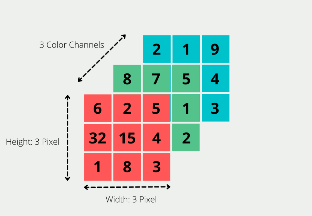
To process an image, we enter each pixel as input into the network. So for an image of size 200x200x3 (i.e. 200 pixels on 200 pixels with 3 color channels, e.g. red, green and blue) we have to provide 200 * 200 * 3= 120,000 input neurons. Then each matrix has a size of 200 by 200 pixels, so 200 * 200 entries in total. This matrix then finally exists three times, each for red, blue, and green. The problem then arises in the first hidden layer, because each of the neurons there would have 120,000 weights from the input layer. This means the number of parameters would increase very quickly as we increase the number of neurons in the Hidden Layer.

This challenge is exacerbated when we want to process larger images with more pixels and more color channels. Such a network with a huge number of parameters will most likely run into overfitting. This means that the model will give good predictions for the training set, but will not generalize well to new cases that it does not yet know.

Additionally, due to a large number of parameters, the network would very likely stop attending to individual image details as they would be lost in sheer mass. However, if we want to classify an image, e.g. whether there is a dog in it or not, these details, such as the nose or the ears, can be the decisive factor for the correct result.

What makes the Convolutional Neural Network different?

For these reasons, the Convolutional Neural Network takes a different approach, mimicking the way we perceive our environment with our eyes. When we see an image, we automatically divide it into many small sub-images and analyze them one by one. By assembling these sub-images, we process and interpret the image. How can this principle be implemented in a Convolutional Neural Network?

The work happens in the so-called convolution layer. To do this, we define a filter that determines how large the partial images we are looking at should be, and a step length that decides how many pixels we continue between calculations, i.e. how close the partial images are to each other. By taking this step, we have greatly reduced the dimensionality of the image.

The next step is the pooling layer. From a purely computational point of view, the same thing happens here as in the convolution layer, with the difference that we only take either the average or maximum value from the result, depending on the application. This preserves small features in a few pixels that are crucial for the task solution.

Finally, there is a fully-connected layer in the Convolutional Neural Network, as we already know it from the normal neural networks. Now that we have greatly reduced the dimensions of the image, we can use the tightly meshed layers. Here, the individual sub-images are linked again in order to recognize the connections and carry out the classification.

Now that we have a basic understanding of what the individual layers of a Convolutional Neural Networkroughly do, we can look in detail at how an image becomes a classification. For this purpose, we try to recognize from a 4x4x3 image whether there is a dog in it.

Detail: Convolution Layer

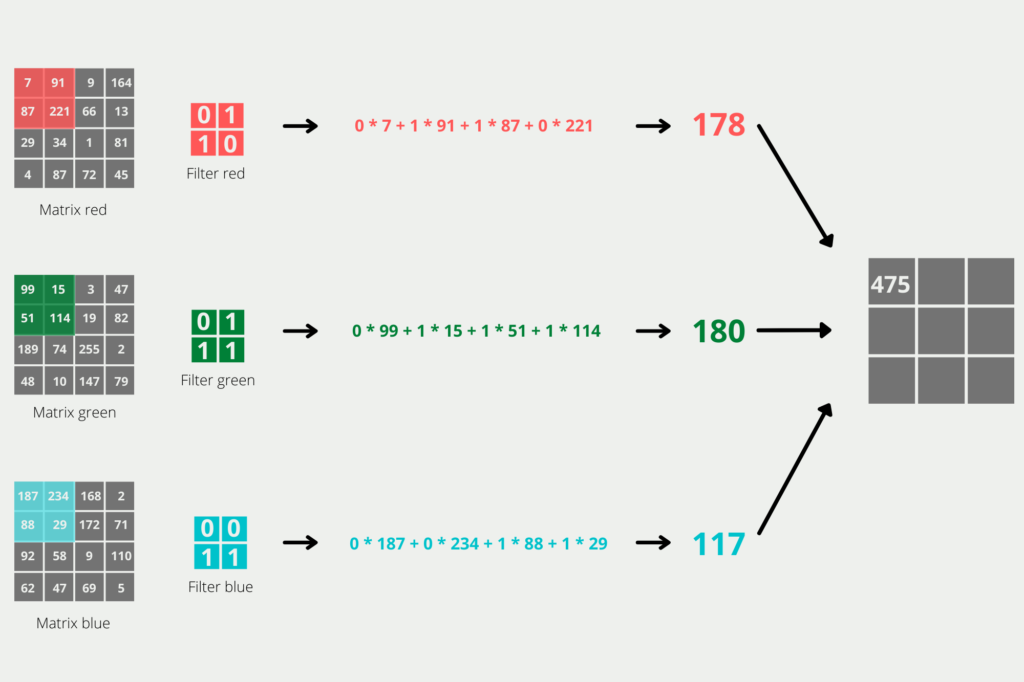
In the first step, we want to reduce the dimensions of the 4x4x3 image. For this purpose, we define a filter with the dimension 2×2 for each color. In addition, we want a step length of 1, i.e. after each calculation step, the filter should be moved forward by exactly one pixel. This will not reduce the dimension as much, but the details of the image will be preserved. If we migrate a 4×4 matrix with a 2×2 and advance one column or one row in each step, our Convolutional Layer will have a 3×3 matrix as output. The individual values of the matrix are calculated by taking the scalar product of the 2×2 matrices, as shown in the graphic.

Detail: Pooling Layer

The (Max) Pooling Layer takes the 3×3 matrix of the convolution layer as input and tries to reduce the dimensionality further and additionally take the important features in the image. We want to generate a 2×2 matrix as the output of this layer, so we divide the input into all possible 2×2 partial matrices and search for the highest value in these fields. This will be the value in the field of the output matrix. If we were to use the average pooling layer instead of a max-pooling layer, we would calculate the average of the four fields instead.

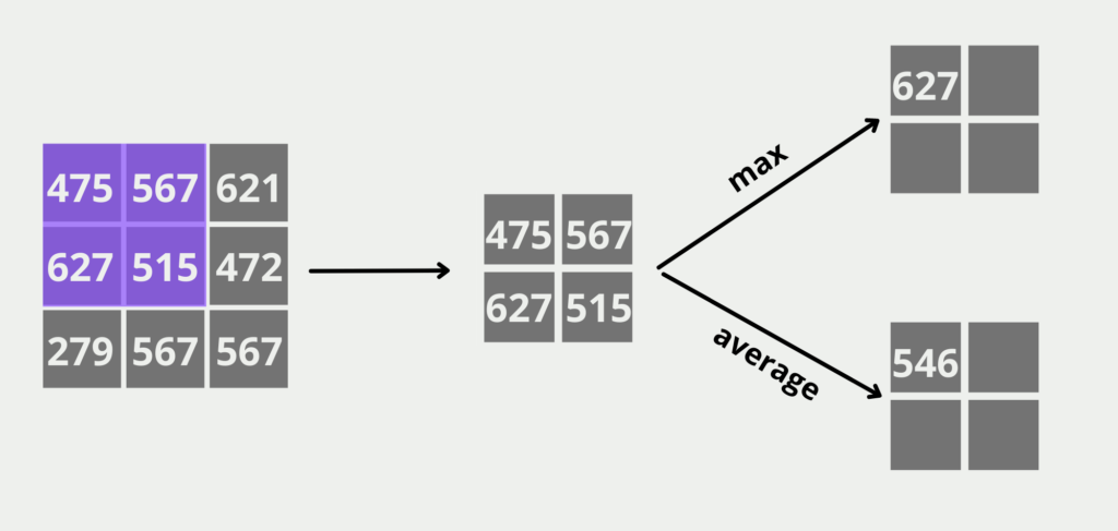
The pooling layer of the Convolutional Neural Network also filters out noise from the image, i.e. elements of the image that do not contribute to the classification. For example, whether the dog is standing in front of a house or in front of a forest is not important at first.

Detail: Fully-Connected Layer

The fully-connected layer now does exactly what we intended to do with the whole image at the beginning. We create a neuron for each entry in the smaller 2×2 matrix and connect them to all neurons in the next layer. This gives us significantly fewer dimensions and requires fewer resources in training.

This layer then finally learns which parts of the image are needed to make the classification dog or non-dog. If we have images that are much larger than our 5x5x3 example, it is of course also possible to set the convolution layer and pooling layer several times in a row before going into the fully-connected Layer. This way you can reduce the dimensionality far enough to reduce the training effort.

How can the training set for Convolutional Neural Networks be increased?

Large data sets are often required for training models in image processing. Especially in the area of supervised learning, where each image needs a label, these are often difficult and expensive to obtain, since they usually have to be classified by hand. Therefore, there are different possibilities in the field of data augmentation to artificially enlarge the data set.

In data augmentation, the existing training data is transformed to create new training examples. The idea is that these new examples are similar enough to the original examples to capture the same underlying patterns but different enough to provide additional information to the network.

Some common transformations used in CNNs for data augmentation are:

• Rotate: Rotating the image by a certain angle can help the network learn rotation-invariant features.
• Mirroring: Rotating the image horizontally or vertically can help the network learn features that cannot be changed.
• Cropping and resizing: Randomly cropping and resizing the image can help the network learn scale-invariant features.
• Color Shifting: Applying random color transformations to the image, such as changing the brightness or contrast, can help the network learn color invariant features.
• Gaussian noise: Adding Gaussian noise to the image can help the network learn features that are robust to noise.
• Elastic deformation: Applying elastic deformation to the image can help the network learn features that are robust to small distortions.

It is important to note that data augmentation should be done in a way that preserves the semantic content of the image. For example, if you rotate an image of a cat horizontally, you still get an image of a cat, but if you rotate an image with text horizontally, you get gibberish.

Overall, data augmentation can be a powerful tool for improving the performance of CNNs, especially when used in combination with other techniques such as regularization and early termination.

What optimization algorithms can be used to train CNNs?

There are several optimization algorithms that can be used to train Convolutional Neural Networks (CNNs), including:

• Stochastic Gradient Descent (SGD): SGD is a popular optimization algorithm used to train CNNs. In this method, the weights of the network are updated based on the gradients of the loss function concerning the weights. The learning rate determines the step size of the weight updates.
• Adagrad: Adagrad is an adaptive optimization algorithm that adjusts the learning rate for each weight based on the historical gradients for that weight. This can be useful in cases where some weights require more updates than others.
• Adadelta: Adadelta is another adaptive optimization algorithm that uses an estimate of the second moment of the gradients to adaptively adjust the learning rate. It was developed to address some of the limitations of Adagrad, such as the decreasing learning rate problem.
• Adam: Adam is a popular adaptive optimization algorithm that combines ideas from Adagrad and RMSprop. It maintains an estimate of the first and second moments of the gradients to adaptively adjust the learning rate.
• Momentum: Momentum is a technique that adds a momentum term to the updates of the weights, which helps the optimization algorithm to move in the same direction as the previous updates. This can help speed up convergence and reduce oscillations.
• Nesterov Accelerated Gradient (NAG): NAG is a variant of momentum where the gradient at a future point in weight space is calculated based on the current momentum. This can help reduce oscillations and accelerate convergence.

Each optimization algorithm has its strengths and weaknesses, and the choice of algorithm depends on the specific problem to be solved and the characteristics of the data set. It is common to try different optimization algorithms and compare their performance against a validation set to select the best algorithm

This is what you should take with you

• Convolutional neural networks are used in image and speech processing and are based on the structure of the human visual cortex.
• Convolutional Neural Networks consist of a convolution layer, a pooling layer, and a fully connected layer.
• Convolutional neural networks divide the image into smaller areas in order to view them separately for the first time.
• This makes convolutional neural networks much more resource-efficient than if we would do such a computation in a Fully-Connected Neural Network.

Other Articles on the topic of Convolutional Neural Network

• An explanation of convolutional neural networks and their implementation in Tensorflow can be found here.