The Stochastic Gradient Descent is an algorithm for training Machine Learning models especially deep neural networks. The difference of the Stochastic Gradient Descent compared to the regular gradient method is that the gradient is not calculated from the entire batch, but only from a subset. This can significantly reduce the required computing power, especially in high-dimensional space.

What is the gradient descent method used for?

The goal of artificial intelligence is generally to create an algorithm that can make a prediction as accurately as possible with the help of input values, i.e. that comes very close to the actual result. The difference between the prediction and the reality is converted into a mathematical value by the so-called loss function. The gradient method is used to find the minimum of the loss function because then the optimal training condition of the model is found.

The training of the AI algorithm then serves to minimize the loss function as much as possible in order to have a good prediction quality. The artificial neural network, for example, changes the weighting of the individual neurons in each training step in order to approximate the actual value. In order to be able to specifically address the minimization problem of the loss function and not randomly change the values of the individual weights, special optimization methods are used. In the field of artificial intelligence, the so-called gradient descent method is most frequently used.

Why do we approach the minimum and not just calculate it?

From the mathematical subfield of analysis we know that a minimum or maximum can be determined by setting the first derivative equal to zero and then checking whether the second derivative is not equal to 0 at this point. Theoretically, we could also apply this procedure to the loss function of the artificial neural network and thus calculate the minimum exactly.

In higher mathematical dimensions with many variables, however, the exact calculation is very complex and would take up a lot of computing time and, above all, resources. In a neural network, we can quickly have several million neurons and thus correspondingly several million variables in the function.

Therefore, we use approximation methods to be able to approach the minimum quickly and be sure after a few repetitions to have found a point close to the minimum.

What is the basic idea of Gradient Descent?

Behind the gradient method is a mathematical principle that states that the gradient of a function (the derivative of a function with more than one independent variable) points in the direction in which the function rises the most. Correspondingly, the opposite is also true, i.e. that the function falls off most sharply in the opposite direction of the gradient.

In the gradient descent method, we try to find the minimum of the function as quickly as possible. In the case of artificial intelligence, we are looking for the minimum of the loss function and we want to get close to it very quickly. So if we go in the negative direction of the gradient, we know that the function is descending the most and therefore we are also getting closer to the minimum the fastest.

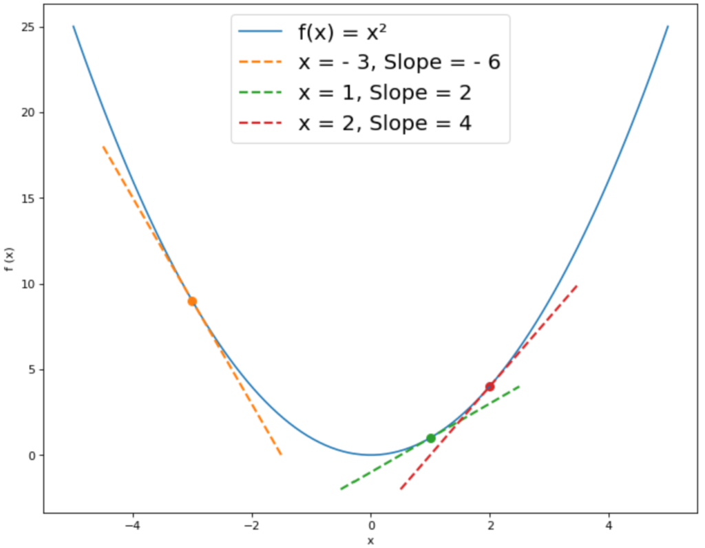
For the function f(x) = x² we have drawn the tangents with the gradient f'(x) at some points. In this example, the minimum is at the point x = 0. At the point x = -3, the tangent has a slope of -6. According to the gradient method, we should move in the negative direction of the gradient to get closer to the minimum, so – (- 6) = 6. This means that the x-value of the minimum is greater than -3.

At the point x = 1, however, the derivative f'(1) has a value of 2. The opposite direction of the gradient would therefore be -2, which means that the x-value of the minimum is less than x = 1. This brings us gradually closer to the minimum.

In short, the gradient method states:

• If the derivative of the function is negative at the point x, we go forward in the x-direction to find the minimum.
• If the derivative of the function is positive at the point x, we go backward in the x-direction to find the minimum.

In the case of a function with more than one variable, we then consider not only the derivative but the gradient. In multidimensional space, the gradient is the equivalent of the derivative in two-dimensional space.

What problems can occur with the gradient descent method?

There are two major problem areas that we may have to deal with when using the gradient method:

• We end up with a local minimum of the function instead of a global one: Functions with many variables very likely do not have only one minimum. If a function has several extreme values, such as minima, we speak of the global minimum for the minimum with the lowest function value. The other minima are so-called local minima. The gradient method does not automatically save us from finding a local minimum instead of a global one. However, to avoid this problem we can test many different starting points to see if they all converge toward the same minimum.

• Another problem can occur when we use the gradient descent method in connection with neural networks and their loss function. In special cases, e.g. when using feedforward networks, it can happen that the gradient is unstable, i.e. it becomes either very large or very small and tends towards 0. With the help of other activation functions of the neurons or certain initial values of the weights one can prevent these effects. However, this is beyond the scope of this paper.
• In the classical method, the computation of the gradient can be very computationally intensive, resulting in higher costs in computing power or more time in training.

What is the Stochastic Gradient Descent?

In the “classical” gradient method, the gradient is calculated after each batch, which is why it is also called batch gradient descent. A batch is a part of the training data, which in many cases has 32 or 64 training instances. First, the predictions for all instances in the batch are calculated and then the weights are changed by backpropagation. This can greatly increase the computing power, especially for complex models, for example in image or speech processing. In these applications, the information is additionally relatively sparse, which means that although the data has many attributes, these also often have the value 0.

The Stochastic Gradient Descent, therefore, provides the approach that the gradient is not calculated from a batch, but for each data point. That means in each iteration only one single data point is used. This reduces the used computing power enormously since the remaining batch does not have to be kept in the working memory. This is called Stochastic Gradient Descent, because in each training step the gradient is only an approximation of the actual gradient.

What are the advantages and disadvantages of the Stochastic Gradient Descent?

The use of Stochastic Gradient Descent offers the following advantages:

• Efficiency: By using a smaller sample, the required computing power is significantly reduced and costs can be saved in training.
• Training Time: For larger data sets, Stochastic Gradient Descent can lead to faster convergence, as parameters are adjusted much more frequently than when processed in batch. However, as we will see in a moment, this point can tend in either direction.
• Ease of use: The concept of Stochastic Gradient Descent is comparatively simple and can therefore be programmed and modified very quickly.

However, Stochastic Gradient Descent should only be used if batch processing would not be possible, because it has the following disadvantages, among others:

• Noise in training: Due to the imprecise gradient, the path to the minimum of the loss function is much stonier and characterized by noise.
• Training time: Due to greater noise, the training time can also increase compared to the conventional approach. Thus, this point is always dependent on the specific application.
• Hyperparameter: With the Stochastic Gradient Descent, there are significantly more hyperparameters, which must be additionally adjusted to achieve a good result.

How can the Stochastic Gradient Descent be implemented in Python?

Scikit-Learn already offers a simple function with the help of which the Stochastic Gradient Descent can be implemented without much custom programming. Depending on the application, you can choose between a classifier and a regression:

from sklearn.linear_model import SGDClassifier

clf = SGDClassifier(loss="hinge", penalty="l2", max_iter=5)

For training purposes, there is no need to specify additional parameters that would not be required anyway, such as the loss function.

This is what you should take with you

• The Stochastic Gradient Descent is a variation of the “classic” Batch Gradient Descent and differs in that not a subset of the data set is used to calculate the gradient, but only a single data set.
• It is mainly used when training text or image classifications, where the data sets are often very large and a lot of memory is required. Stochastic Gradient Descent can save considerable computing power, since the complete batch does not have to be loaded into memory. This makes the training cheaper or even possible with the given resources.
• One of the disadvantages of the Stochastic Gradient Descent is that significantly more noise can occur during training, which leads to a slower training time since the path of the loss function to the minimum is significantly stonier.

Other Articles on the Topic of Stochastic Gradient Descent

The documentation in Scikit-Learn for the Stochastic Gradient Descent can be found here.