Logistic regression is a special form of regression analysis that is used when the dependent variable, i.e. the variable to be predicted, can only take on a certain number of possible values. This variable is then also referred to as being nominally or ordinally scaled. Logistic regression provides us with a probability of assigning the data set to a class.

What are possible research questions for logistic regression?

In use cases, it is actually very common that we do not want to predict a concrete numerical value, but simply determine in which class or range a data set falls. Here are a few classic, practical examples for which logistic regression can be used:

• Politics: Which of the possible five parties will a person vote for if there were elections next Sunday?
• Medicine: Is a person “susceptible” or “not susceptible” to a certain disease depending on some medical parameters of the person?
• Business: What is the probability of buying a certain product depending on a person’s age, place of residence, and profession?

How does a logistic regression work?

In linear regression, we tried to predict a concrete value for the dependent variable instead of calculating a probability that the variable belongs to a certain class. For example, we tried to determine a student’s concrete exam grade as a function of the hours the student studied for the subject. The basis for the estimation of the model is the regression equation and, accordingly, the graph that results from it.

Example: We want to build a model that predicts the likelihood of a person buying an e-bike, depending on their age. After interviewing a few subjects, we get the following picture:

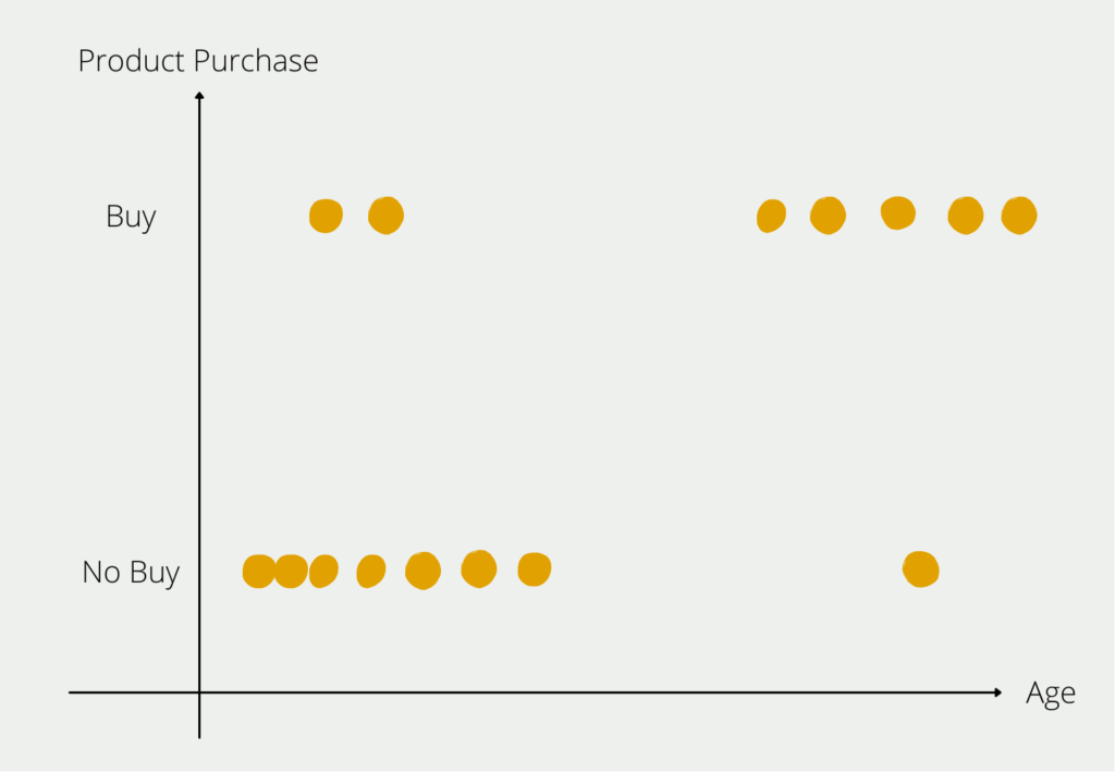
From our small group of respondents, we can see the distribution that young people for the most part have not bought an e-bike (bottom left in the diagram), and older people in particular are buying an e-bike (top right in the diagram). Of course, there are outliers in both age strata, but the majority of respondents conform to the rule that the older you get, the more likely you are to buy an e-bike. We now want to prove this rule, which we have identified in the data, mathematically.

To do this, we have to find a function that is as close as possible to the point distribution that we see in the diagram and, in addition, only takes on values between 0 and 1. Thus, a linear function, as we have used it for the linear regression, is already out of the question, since it lies in the range between -∞ and +∞. However, there is another mathematical function that meets our requirements: the sigmoid function.

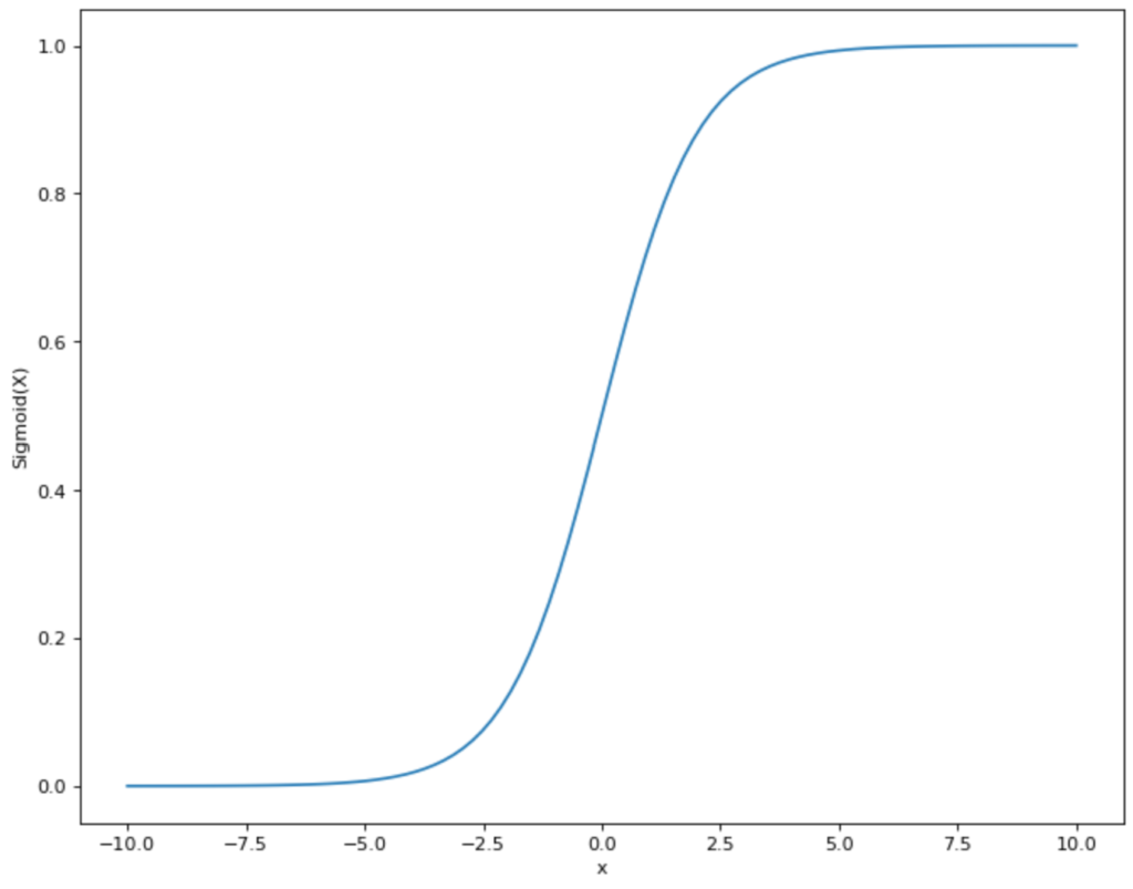
The functional equation of the sigmoid graph looks like this:

\(\) \[S(x) = \frac{1}{1+e^{-x}}\]

Or for our example:

\(\) \[P(\text{Purchase E-Bike})) = \frac{1}{1+e^{-(a + b_1 \cdot \text{Age})}}\]

Thus, we have a function that gives us the probability of buying an e-bike as a result and uses the age of the person as a variable. The graph would then look something like this:

In practice, you often don’t see the notation we used. Instead, one rearranges the function so that the actual regression equation becomes clear:

\(\) \[logit(P(\text{Purchase E-Bike}) = a + b_1 \cdot \text{Age}\]

How to interpret a Logistic Regression?

The correlations between independent and dependent variables obtained in logistic regression are not linear and thus cannot be interpreted as easily as in linear regression.

Nevertheless, a basic interpretation is possible. If the coefficient before the independent variable (age) is positive, then the probability of the sigmoid function also increases as the variable increases. In our case, this means that if b1 is positive, the probability of buying an e-bike also increases with increasing age. The opposite is also true, of course, so if b1 is positive, the probability of e-bike purchase also decreases with decreasing age.

Furthermore, comprehensible interpretations with a logistic regression are only possible with great difficulty. In many cases, one calculates the so-called odds ratio, i.e. the ratio of the probability of occurrence and the probability of non-occurrence:

\(\) \[odds = \frac{p}{1-p}\]

If you additionally form the logarithm from this fraction, you get the so-called logit:

\(\) \[z = Logit = ln (\frac{p}{1-p})\]

This looks confusing. Let’s go back to our example to bring more clarity here. Assuming our example we get the following logistic regression equation:

\(\) \[logit(P(\text{Purchase E-Bike})) = 0.2 + 0.05 \cdot \text{Age}\]

This function can be interpreted linearly, so one year increases the logit(p) by 0.05. The logit(p) is according to our definition nothing else than ln(p/(1-p)). So if ln(p/(1-p)), increases by 0.05, then p/(1-p), increases by exp(0.05) (Note: The logarithm ln and the e-function (exp) cancel each other). Thus, with every year that one gets older, the chance (not probability!) of buying e-bike increases by exp(0.05) = 1.051, i.e. by 5.1 percent.

How to evaluate logistic regression?

Logistic regression is a widely used statistical method for binary classification problems where the goal is to predict the probability of an event occurring (e.g., whether a customer will buy a product or not) based on a set of input characteristics. To evaluate the performance of a logistic regression model, several metrics can be used.

• Confusion Matrix: A confusion matrix is a table that summarizes the performance of a binary classification model. It shows the number of true positives (TP), false positives (FP), true negatives (TN), and false negatives (FN) in tabular form.
• Accuracy: Accuracy is the most commonly used metric to evaluate the performance of a logistic regression model. It is defined as the ratio between the number of correct predictions and the total number of predictions. However, precision can be misleading if the classes are unbalanced.
• Precision: Precision is the ratio between the number of correct positive predictions and the total number of positive predictions (i.e., correct positive predictions plus false positive predictions). It measures the proportion of positive predictions that are actually correct.
• Recall: Recall is the ratio of the number of true positive predictions to the total number of actual positive predictions (i.e., true positive predictions plus false negative predictions). It measures the proportion of true positive instances that were correctly predicted.
• F1 Score: The F1 score is the harmonic mean of Precision and Recall. It is a single metric that combines both Precision and Recall and provides a balanced measure of both.
• ROC Curve: The Receiver Operating Characteristic (ROC) curve is a graphical representation of the performance of a binary classification model at various classification thresholds. It plots the true positive rate (TPR) against the false positive rate (FPR) for different thresholds.
• AUC value: The area under the ROC curve (AUC) is a scalar value that summarizes the performance of a binary classification model across all classification thresholds. It provides an aggregate measure of the model’s ability to distinguish between positive and negative instances.

In summary, evaluating a logistic regression model involves the use of multiple metrics, each of which provides a different perspective on the model’s performance. The choice of metrics depends on the specific requirements of the application and the trade-off between precision and recall.

How to deal with unbalanced data?

Dealing with imbalanced data is a common challenge in machine learning, and is particularly relevant when working with logistic regression models. In many real-world scenarios, one of the classes of interest may be underrepresented in the data, resulting in a biased model that performs poorly on that class.

There are several techniques for dealing with imbalanced data when working with logistic regression models:

• Resampling: This involves either oversampling the minority class or undersampling the majority class to balance the data set. However, this approach can lead to overfitting or loss of important information.
• Cost-sensitive learning: In this approach, different costs are assigned to the misclassification of different classes. By increasing the cost of misclassifying the minority class, the model is encouraged to favor the correct classification of that class.
• Ensemble methods: Ensemble methods such as bagging, boosting, or stacking can be effective for dealing with imbalanced data. These methods combine multiple logistic regression models to improve the overall performance of the model.
• Synthetic data generation: This involves generating new data points for the minority class using techniques such as SMOTE (Synthetic Minority Over-sampling Technique). This can help balance the data set and improve the performance of the model.
• Algorithm selection: In some cases, a logistic regression model may not be the best algorithm for unbalanced data. Other algorithms, such as decision trees, random forests, or support vector machines, may perform better on unbalanced data sets.

It is important to carefully evaluate the performance of logistic regression models on unbalanced data and choose the appropriate technique to handle the imbalance. Evaluation metrics for imbalanced data sets should also be carefully selected, e.g., the area under the receiver operating characteristic (ROC) curve, the precis

This is what you should take with you

• Logistic regression is used when the outcome variable is categorical.
• We use the sigmoid function as the regression equation, which can only take values between 0 and 1.
• Logistic regression and its parameters are not as easy to interpret as linear regression.

Other Articles on the Topic of Logistic Regression

• The University of Zurich has an interesting paper explaining logistic regression in detail and with examples.