Q-learning is an algorithm from the field of reinforcement learning that attempts to predict the next best action based on the agent’s current environment. It is mainly used for learning games in which a promising strategy is to be developed.

What is Reinforcement Learning?

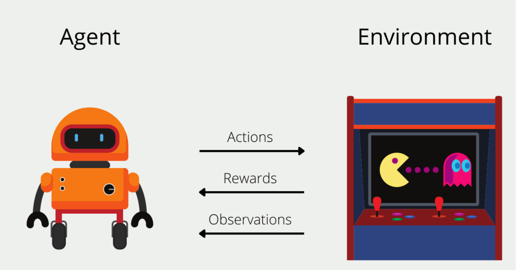
Reinforcement Learning models are to be trained to make a series of decisions independently. Let us assume that we want to train such an algorithm, the so-called agent, to play the game PacMan as successfully as possible. The agent starts at an arbitrary position in the game field and has a limited number of possible actions it can perform. In our case, this would be the four directions (up, down, right, or left) that it can go on the playing field.

The environment in which the algorithm finds itself in this game is the playing field and the movement of ghosts, which must not be encountered. After each action, for example, go up, the agent receives direct feedback, the reward. In PacMan, these are either getting points or encountering a ghost. It can also happen that after an action there is no direct reward, but it takes place in the future, for example in one or two more moves. For the agent, rewards that are in the future are worth less than immediate rewards.

Over time, the agent develops a so-called policy, i.e. a strategy of actions that promises the highest long-term reward. In the first rounds, the algorithm selects completely random actions, since it has not yet been able to gain any experience. Over time, however, a promising strategy emerges.

What is Q-Learning?

Q-Learning is a reinforcement learning algorithm that tries to maximize the reward in each step depending on possible actions. This algorithm is said to be “model-free” and “off-policy”.

“model-free” means that the algorithm does not resort to modeling a probability distribution, i.e., it tries to predict the response of the environment. A “model-based” approach in a game, such as PacMan, would try to learn which reward and which new state it can expect before deciding on an action. A “model-free” algorithm, on the other hand, completely ignores this and rather learns according to the “trial and error” principle by choosing a random action and only then evaluating whether it was successful or not.

The property “off-policy” means that the model does not follow any policy at first. This means that the model decides at each point in time which action is the best in the current environment, regardless of whether this fits the previously followed policy or not. This means that there are no strategies that involve multiple moves, but rather that the model thinks in steps that involve only a single action.

How does the process work?

In the course of the Q-learning algorithm, various steps are run through. The focus is on the q-table, which helps the algorithm to select the correct actions. The number of rows is the possible states of the game, e.g. for PacMan encountering a ghost or collecting points. The number of columns is the actions that can be performed, i.e. the directions in which the figure can be moved.

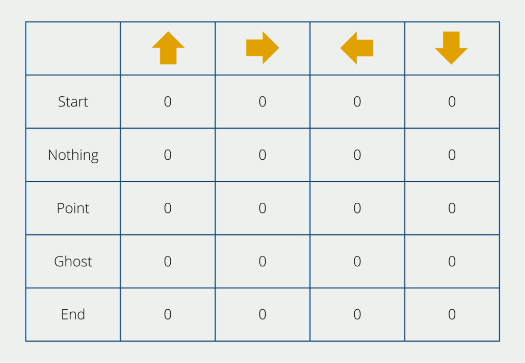
In the beginning, the values of the table are set to 0. In the course of the training, these values change constantly. The following steps are run through during learning:

Creating the q-table

The table, as we have already seen, is created and the individual values must be filled, i.e. initialized. In our case, we write a zero in each field, but other methods can also be used to initialize the fields.

Action selection

Now the algorithm starts to select one of the possible actions in its respective state (i.e. Start at the beginning). The algorithm uses two different approaches:

1. Exploration: In the beginning, the model does not yet know any Q-values and selects actions randomly. In this way, it explores the individual statuses and recognizes new procedures that would otherwise have remained undiscovered.
2. Exploitation: During the Exploitation phase, the model tries to exploit the knowledge from the Exploration phase. If the q-table already contains reliable values, the algorithm selects the action for each state that promises the highest future reward.

How often the model should be in exploration or exploitation can be set via the so-called epsilon value. It decides the ratio of the two types of choice of actions.

Overwrite the q-values

With each action that the agent chooses during Q-learning, the values in the q-table also change. This happens until a predetermined endpoint is reached and thus the game comes to an end. In PacMan, this point is reached either when you encounter a ghost or when you have collected all points in the game field. The next game can then already be started with the already learned q-values.

After the agent has chosen an action in its initial state, it receives a reward. The q-value for the field of the corresponding state and action is then calculated using the following formula:

\(\) [Q(S_{t}, A_{t}) = (1 – alpha) cdot Q(S_{t}, A_{t}) + alpha cdot (R_{t} + lambda cdot max_{alpha} Q(S_{t + 1}, alpha))]

These are the meanings of the individual components:

• S stands for the state. The index t is the current state and the index t+1 is the future state.
• A is the action that the algorithm chooses.
• R is the reward, i.e. the effect of the action taken. This can be either positive, such as an extra point, or negative, such as encountering a ghost.
• α is the learning rate, as we already know it from other models in Machine Learning. It decides how much the now calculated value, overwrites the already existing value of the table.
• λ is the discount factor, i.e. a factor that values future events less strongly than present ones. This factor leads to the algorithm weighing short-term rewards higher than future ones.

This loop is executed as often as defined in the code or terminated early if a criterion is reached. The resulting q-table is then the result of the Q-learning algorithm and can then be queried.

Where does the name come from?

The Q in Q-Learning stands for quality. This measures how valuable the next action is to receive a reward in the following step or in the future. The q-values come from the so-called q-table and are calculated using a given formula. The q-value decides whether an action will be executed next.

What is the difference between Q-Learning and G-Learning?

Both Q-learning and G-learning are algorithms that are used in the field of reinforcement learning to find optimal strategies for sequential, i.e. consecutive, decisions. In this section, we will take a closer look at the similarities and differences between the two approaches.

In Q-learning, the focus is on so-called state-action pairs, for which a so-called Q-value is estimated to find an optimal strategy. To do this, an action value function \(Q(s,a)\) is learned, which returns an expected cumulative reward for each pair of state and action. Through an iterative process, the Q values are updated based on the observed rewards and the subsequent states of the system. The temporal difference method is used for this.

The focus of Q-learning is therefore the evaluation of the current state together with the optimal next action. This provides the agent with information about which optimal action he or she should perform next. The action with the highest Q value is simply selected. This approach is particularly useful when a specific strategy is to be learned and there is also a discrete action space, i.e. a well-defined set of actions available, such as the movement options in Pacman. In practice, Q-learning is mainly used in robotics or when learning games.

G-learning, on the other hand, attempts to estimate the value of a state directly, without taking into account the possible actions. The state value function only has one input parameter here, namely the state, i.e. \(G(s)\). It returns the expected cumulative reward for each state. Analogous to Q-learning, the TD method for iterative updates is used to estimate the function. However, it only uses the values of the states for these updates and not the actions. G-learning is particularly suitable for applications that do not have a well-defined action space and where the reward of the state plays a major role, such as in financial analysis or medical decisions.

As we have seen, the choice between G-learning and Q-learning depends on the application and the goals that the model is intended to achieve. If the focus is on finding an optimal strategy and determining an optimal action for each state, Q-learning should be preferred. If, on the other hand, different states are to be assessed and compared, G-learning is more suitable.

This is what you should take with you

• Q-learning is a powerful reinforcement learning algorithm used to solve sequential decision-making problems.
• It learns an action-value function (Q-values) to estimate the expected cumulative rewards of state-action pairs.
• Q-learning utilizes the temporal difference (TD) method to iteratively update Q-values based on observed rewards and subsequent states.
• The algorithm enables agents to make optimal decisions by selecting actions with the highest Q-values in each state.
• Q-learning is well-suited for applications with discrete action spaces, such as game-playing or robotics.
• It has been successfully applied in various domains, including autonomous driving, game AI, and robotics.
• Q-learning provides a framework for learning and optimizing policies in complex environments.
• By balancing exploration and exploitation, Q-learning allows agents to improve their decision-making over time.
• Understanding Q-learning and its underlying principles is crucial for mastering reinforcement learning techniques.
• Further research and advancements in Q-learning continue to expand its applications and improve its performance.

Other Articles on the Topic of Q-Learning

This contribution to the publication TowardsDataScience explains the Q-learning algorithm in detail and implements it in Python.