What is the ARIMA Model?

The abbreviation ARIMA stands for AutoRegressive Integrated Moving Average and refers to a class of statistical models used to analyze time series data. This model can be used to make predictions about the future development of data, for example in the scientific or technical field. The ARIMA method is primarily used when there is a so-called temporal autocorrelation, i.e. simply put, the time series shows a trend.

In this article, we will explain all aspects related to ARIMA models, starting with a simple introduction to time series data and its special features, until we train our own model in Python and evaluate it in detail at the end of the article.

What is time series data?

Time series data is a special form of data set in which the measurement has taken place at regular, temporal intervals. This gives such a data collection an additional dimension that is missing in other data sets, namely the temporal component. Time series data is used, for example, in the financial and economic sector or in the natural sciences when the change in a system over time is measured.

The visualization of time series data often reveals one or more characteristics that are typical for this type of data:

Trends: A trend describes a long-term pattern in the data such that the measurement points either increase or decrease over a longer period of time. This means that despite short-term fluctuations, an overall direction of travel can be recognized. A healthy company, for example, records sales growth over several years, although it may also have to record sales declines in individual months.
Seasonality: Seasonality refers to recurring patterns that occur at fixed intervals and are therefore repeated. The duration and frequency of seasonality depends on the data set. For example, certain patterns can repeat themselves daily, hourly or annually. The demand for ice cream, for example, is subject to great seasonality and usually increases sharply in summer, while it decreases in winter. This behavior therefore repeats itself every year. Seasonality is characterized by the fact that it occurs within a fixed framework and is therefore easy to predict.
Cycle: Although cycles are also fluctuations in the data, they do not occur as regularly as seasonal changes and are often of a longer-term nature. In the case of economic time series, these fluctuations are often linked to economic cycles. In the phase of an economic upswing, for example, a company will record significantly stronger economic growth than during a recession. However, the end of such a cycle is not as easy to predict as the end of a season.
Outliers: Irregular patterns in time series data that follow neither a seasonality nor a trend are called outliers. In many cases, these fluctuations are related to external circumstances that are difficult or impossible to control. These changes make it difficult to accurately predict future developments. A sudden natural disaster, for example, can have a negative impact on the company’s sales figures because delivery routes are flooded.
Autocorrelation: Autocorrelation describes the phenomenon where past data points in a series of measurements are correlated with future data, i.e. they depend on each other. This dependency can help with the prediction of new values. A measurement series of temperature values has an autocorrelation, as the current temperature depends on the temperature two minutes ago.

What is ARIMA?

ARIMA models (AutoRegressive Integrated Moving Average) are statistical methods for analyzing time series data and predicting future values. They are able to recognize the temporal structures that have arisen and include them in the forecasts.

The abbreviation already describes the three main components that make up the model. These components are explained in more detail below and illustrated using the example of a sales forecast.

Autoregression (AR): The autoregressive component (AR) of the model uses past values to make future forecasts. This means that the extent of the past data points is taken into account directly for the estimate and autocorrelation is therefore taken into account.

Example: When predicting future sales development, it can be important to consider the patterns and trends from previous periods in order to incorporate their information. If sales have risen in the last three months, the AR element could indicate that sales will also rise this month, as there is currently an upward trend.
Model: In the ARIMA model, the autoregressive component is characterized by the variable \( p \), which is also called lag. This parameter defines how many previous periods are used to predict the next value. A model with \( p = 2 \) therefore uses the two previous months to estimate sales in the coming month.

Integrated (I): The I component stands for “integrated” and refers to the process of differentiation. In many time series data, trends and patterns ensure that the values are not stationary, i.e. their statistical properties, such as the mean or variance, change over time. However, stationarity is a fundamental property for training powerful statistical models. Therefore, differencing can help to remove any trends and patterns from the data to make the dataset stationary.

Example: If there is an increasing pattern in sales, it can be helpful to differentiate the values and thus only look at the changes from month to month instead of the absolute values. This makes it easier to recognize the underlying pattern and quantify it.
Model: The parameter \( d \) is used in the model itself and specifies how often the differentiation must be applied to make the data stationary. A model with \(d = 1 \) must be differentiated once accordingly. In many cases, a single differentiation is sufficient to make the data set stationary.

Moving average (MA): The moving average refers to the dependency of errors or residuals over time. This component therefore takes into account the errors that have occurred in the prediction of previous values and includes them in the current estimate. Otherwise, a large error in one month could have a negative impact on the following months and increase even further.

Example: If the turnover in the current month was estimated as too high, this error should be included for the further forecast so that the current forecast is not affected and is also estimated as too high.
Model: The parameter \( q \) can be used to define how many previous errors are taken into account for the current estimate.

The ARIMA model is a powerful method that consists of three main components and includes the past values, the stationarity of the data and the previous errors in the estimate.

What does stationarity of data mean?

Stationarity plays a crucial role in time series analysis, as it is assumed by many models, such as the ARIMA model. Many time series contain underlying patterns and trends, such as a continuous increase, which ensure that the statistical properties, such as the mean or variance, change over time. However, in order to achieve reliable predictions, it must be ensured that the data set has stationary properties, which is why we will look at the concept in more detail in this section.

A time series is stationary if the statistical properties remain constant over time. In particular, the following characteristic values are considered:

Constant mean: The arithmetic mean of the data set must remain constant over time and should therefore neither increase nor decrease.
Constant variance: The spread around the mean value is always the same over time. The data is therefore not sometimes closer and sometimes further away from the mean value.
Constant autocorrelation: The correlation between two different data points depends solely on the distance between the two points and not on time.

Only if these properties are fulfilled can it be assumed that previous patterns also reliably predict future patterns, because in a stationary time series the relationships between the data points also remain stable over time.

To check stationarity, a simple visual representation of the data can help in the first step to identify trends or patterns that prevent stationarity. If, on the other hand, a seasonality of the time series can be recognized, then the data is clearly not stationary. However, to be on the safe side, the so-called Augmented Dickey-Fuller test (ADF test) can also be used.

If the time series turns out to be non-stationary, it must first be made stationary in order to be able to use statistical models such as ARIMA. One of the most effective methods for this is differencing. In this process, the differences between successive data points are calculated in order to remove the underlying trend from the data. As a result, it is no longer the absolute values of the time series that are considered, but their changes.

The first differentiation can be calculated using the following formula:

\(\)\[ y_t^\prime=y_t-y_{t-1} \]

In some cases, a single differentiation may not be sufficient and multiple differentiations must be made. The same procedure is repeated with the already differentiated values until the stationarity of the data is given.

How do you build an ARIMA model?

Now that we have taken a closer look at the structure of the ARIMA model, we can begin to build the model. The focus here is on the three main components and choosing the right size for their parameters. Only if these are chosen correctly can a good and efficient model be trained.

The following parameters must be selected correctly based on the data set:

The parameter \(p\) (autoregressive order) determines the number of lags that must be taken into account for the autoregression. With \( p = 2 \), for example, the last two data points are used to predict the future value.
The parameter \( d \) (differentiation) determines how often the time series must be differentiated so that the data set is stationary, i.e. the statistical key figures are constant. Usually \( d = 1 \) can be set here, as in many cases one differentiation is sufficient to remove trends and patterns and thus make the time series stationary.
The parameter \( q \) (moving average order) defines the number of past errors used in the model.

In order to find the correct values for the parameters \(p\) and \(q\), graphical tools can be used to help with the selection.

Autocorrelation function (ACF)

This function shows the correlation of a time series with the various lags. This makes it possible to see graphically whether and to what extent a value in the time series is correlated with the previous lags.

If the correlation drops only slowly, as in the graph above, then this may indicate that a model with a certain \(p\) value may be suitable, which can be selected more precisely using the following function. However, if there is a sharp drop between two lags, this would suggest a moving average model.

Partial autocorrelation function (PACF)

The PACF shows the partial correlation between two data points and has already removed the influence of the points in between. In concrete terms, this means that a break in the PACF after a certain lag is a good indicator of a first \(p\) value that can be tested.

In this graph, the first two lags show a significant correlation and after the second lag there is a rapid drop. The value \(p = 2\) should therefore be set for the model based on the data set. Due to the fact that the ACF function only drops very weakly, a model with \(q = 0\) or \(q = 1\) could be tested.

Before the model can be trained, the data must be made stationary. To do this, you can differentiate the time series and in many cases already obtain stationary data. These are the most important steps to be able to train an ARIMA model.

How to implement the ARIMA model in Python?

An ARIMA model can be implemented in Python using the pmdarima library, which already offers a ready-made function for this. In this example, we use the data set “Air Passengers”, which contains a time series on the monthly passenger numbers of international airlines. We read this via the URL of the corresponding data set from GitHub:

For each month from January 1949 to 1960, we see the number of passengers and their development:

To be able to work with the data, the month specification is converted into a date specification, as we cannot work with a string.

In addition, the month is used as the index of the DataFrame to make it easier to work with the data. easier to work with the data.

Now that the data is sufficiently prepared, we can use the ACF and PACF function to look at the autocorrelation to determine the parameters. As we will see later, this step is actually no longer necessary as the auto_arima function automatically finds the best parameters, but it helps to get a basic understanding of the information.

The two functions can be imported and created using Matplotlib and the modules from statsmodels:

To instantiate an ARIMA model, we use the auto_arima function, which automatically selects the optimal parameters by passing it the data. We also set the seasonal parameter to true, as we expect seasonality in the data. The default value is also true, so we don’t actually need to define it additionally. The parameter m can be used to define the number of observations for a cycle. As we assume seasonality that is repeated annually, i.e. every twelve months, we set the parameter m = 12.

Now we fit the instantiated model to the data and find the optimal parameters. For our data set, the optimal parameters are (2, 1, 1), i.e. \(p = 2\), \(d = 1\) and \(q = 1\).

This model can then be used to make statements. The .predict() function is used for this and the number of periods for which a prediction is to be made is defined:

To assess the quality of the forecasts, we can look at the graphical representation of the curve. The forecasts appear to be accurate as the seasonality continues and the upward trend in passenger numbers is maintained.

These simple steps can be used to train an ARIMA model in Python. Thanks to the automatic search for the optimum parameters, only the data set needs to be well prepared and the seasonality possibly adjusted. Finally, the model should be evaluated with suitable key figures. In the next section, we will take a closer look at which ones can be used for this.

How can a model be evaluated?

Once we have trained the ARIMA model, it is crucial to evaluate its performance sufficiently to ensure that it represents the underlying time series well enough. To perform this model evaluation, there are various metrics and analyses that can be calculated.

Residual analysis

The purpose of the residual analysis is to examine the errors in the predictions more closely.Ideally, these are like “white noise” and therefore no longer exhibit any systematic patterns.In addition, a “good” error has a mean value of 0.

The autocorrelation function (ACF) already presented can be used to examine whether the residuals show a correlation with one’s own past values. The residuals of the model are obtained using model.resid() and can then be converted into a graph using statsmodels.

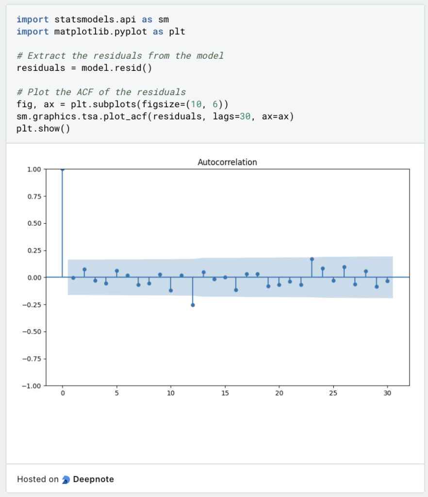
As can be seen in the graph, there is no really significant autocorrelation between the residuals.

Validation of the model

In addition, as with other models, the mean square error and the mean absolute error can be calculated in order to assess the accuracy of the predictions.A smaller error means a higher accuracy of the predictions.To do this, the data set is split into training and test sets in order to check how the model reacts to unseen data that was not used for training. For a small data set, for example, an 80/20 split is a good idea, so that 80% of the data is used for training and the remaining 20% of the data is left for testing.

The diagram shows that the prediction in red follows the course of the actual data fairly accurately, but does not always hit the values exactly, so that a not inconsiderable error remains. For better results, the parameters could be further optimized and additional training runs could be carried out.

What is the seasonal ARIMA model?

Over the years, several extensions of ARIMA have been developed that further adapt the basic model and optimize it for more specific applications. One of these is the SARIMA model, i.e. the Seasonal ARIMA, which offers the possibility of taking seasonal patterns into account in the forecast. There are some additional parameters that capture these seasonal cycles:

P: Here, too, the parameter \(p\) stands for the autoregressive order. However, it is about the extent to which previous seasonal values influence current seasonal values.
D: This parameter also measures how often the data must be differentiated in order to make the data stationary and therefore free of seasonal trends.
Q: The parameter \(q\) takes into account the random errors from previous seasonal periods.
S: This parameter is new and describes how many data points a single season contains.

The SARIMA model should be used above all when the time series are not only subject to trends, but also go through regularly recurring cycles. An example of this could be the energy consumption of all households, which is subject to seasonal fluctuations, for example because more light is needed in winter and therefore more electricity is consumed than in summer.

In which applications is ARIMA used?

ARIMA models are a powerful way of effectively analyzing and predicting time series. In a wide variety of applications, it is important to be able to make predictions about the future as accurately as possible. The most popular ARIMA applications include, for example

Financial market: ARIMA models are used to predict financial time series, such as stock or currency prices.
Energy and utility companies: In order to provide sufficient energy for customers, energy companies must have an early estimate of future consumption. ARIMA models or even SARIMA models are very suitable for this, as they can incorporate seasonal factors and trends into the forecast.
Health & medicine: In the healthcare industry, time series on cases of illness or hospital visits are analyzed in order to adjust the system to future stresses and to have the appropriate medication in stock at an early stage.
Weather forecasting: ARIMA models are also used to forecast weather variables such as temperature or precipitation. These help meteorologists to make accurate forecasts at an early stage and thus, for example, to issue timely warnings of extreme weather events.

ARIMA models are a useful tool for analyzing time series data and can be used in a wide variety of applications.

This is what you should take with you

ARIMA stands for AutoRegressive Integrated Moving Average and is a way of analyzing and predicting time series.
To use this method, it is important that the time series is stationary, i.e. contains constant statistical parameters. Differentiation can be used for this purpose.
In Python, the statsmodels library can be used to train an ARIMA model. The advantage of this implementation is that the optimum parameters are set automatically and do not have to be determined in advance.
To evaluate the model, either the so-called residual analysis can be used or the performance on the test set can be analyzed using cross-validation.
For seasonal data that depends on the seasons, for example, a variant of ARIMA, the so-called SARIMA model, can be used.