A backpropagation algorithm is a tool for improving the neural network during the training process. With the help of this algorithm, the parameters of the individual neurons are modified in such a way that the prediction of the model and the actual value match as quickly as possible. This allows a neural network to deliver good results even after a relatively short training period.

This article joins the other posts on Machine Learning basics. If you don’t have any background on the topic of neural networks and gradient descent, you should take a look at the linked posts before reading on. We will only be able to touch on these concepts briefly. Machine Learning in general is a very mathematical topic. For this explanation of backpropagation, we will try to avoid mathematical derivations as much as possible and just give a basic understanding of the approach.

How do Neural Networks work?

Neural networks consist of many neurons organized in different layers that communicate and are linked to each other. In the input layer, the neurons are given various inputs for computation. The network should be trained so that the output layer, the last layer, makes a prediction based on the input that is as close as possible to the actual result.

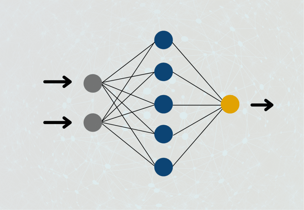
The so-called hidden layers are used for this purpose. These layers also contain many neurons that communicate with the previous and subsequent layers. During training, the weighting parameters of each neuron are changed so that the prediction approximates reality as closely as possible. The backpropagation algorithm helps us decide which parameter to change so that the loss function is minimized.

What is the Gradient Descent Method?

The gradient method is an algorithm from mathematical optimization problems, which helps to approach the minimum of a function as fast as possible. One calculates the derivative of a function, the so-called gradient, and goes in the opposite direction of this vector because there is the steepest descent of the function.

If this is too mathematical, you may be familiar with this approach from hiking in the mountains. You’ve finally climbed the mountaintop, taken the obligatory pictures, and enjoyed the view sufficiently, and now you want to get back to the valley and back home as quickly as possible. So you look for the fastest way from the mountain down to the valley, i.e. the minimum of the function. Intuitively, one will simply take the path that has the steepest descent for the eye, because one assumes that this is the fastest way back downhill. Of course, this is only figuratively speaking, since no one will dare to go down the steepest cliff on the mountain.

The gradient method does the same with a function. We are somewhere in the function graph and try to find the minimum of the function. Contrary to the mountain example, we have only two possibilities to move in this situation. Either in the positive or negative x-direction (with more than one variable, i.e. a multi-dimensional space, there are of course correspondingly more directions). The gradient helps us by knowing that the negative direction of it is the steepest function descent.

What is the Gradient Descent in Machine Learning?

The function that interests us in machine learning is the loss function. It measures the difference between the prediction of the neural network and the actual result of the training data point. We also want to minimize this function, since we will then have a difference of 0. This means our model can accurately predict the results of the data set. The adjusting screws to get there are the weights of the neurons, which we can change to get closer to the goal.

In short: During the training, we get the loss function whose minimum we try to find. For this purpose, we calculate the gradient of the function after each repetition and go in the direction of the steepest descent of the function. Unfortunately, we do not know yet which parameter we have to change and by how much to minimize the loss function. The problem here is that the gradient procedure can only be performed for the previous layer and its parameters. However, a deep neural network consists of many different hidden layers whose parameters can theoretically all be responsible for the overall error.

So in large networks, we also need to determine how much influence each parameter had on the eventual error and how much we need to modify them. This is the second pillar of backpropagation, where the name comes from.

How does the Backpropagation Algorithm work?

We’ll try to keep this post as non-mathematical as possible, but unfortunately, we can’t do it completely without it. Each layer in our network is defined by an input, either from the previous layer or from the training dataset, and by an output, which is passed to the next layer. The difference between input and output comes from the weights and activation functions of the neurons.

The problem is that the influence a layer has on the final error also depends on how the following layer passes on this error. Even if a neuron “miscalculates”, this is not so important if the neuron in the next layer simply ignores this input, i.e. sets its weighting to 0. This is mathematically shown by the fact that the gradient of one layer also contains the parameters of the following layer. Therefore, we have to start the backpropagation in the last layer, the output layer, and then optimize the parameters layer by layer forward using the gradient method.

This is where the name backpropagation, or error backpropagation, comes from, as we propagate the error through the network from behind and optimize the parameters.

How does the forward and backward pass work in detail?

The so-called forward pass describes the normal process of a prediction in a neural network from the input layer via the hidden layers to the output layer. During this pass, the inputs in each layer are changed using a linear transformation and then scaled into a predefined numerical range using the activation function. When the output is finally reached, the values of the last layer are compared with the target value from the data set and the deviation, i.e. the loss or error is calculated.

With the backward pass, this process is somewhat more complex. The aim here is to adjust the weights of the individual neurons in such a way that the error is minimized, thereby further increasing the accuracy of the model predictions.

The gradient of the loss function comes into play to determine the level and direction of the adjustment. This is calculated using the mathematical chain rule and contains the derivative of the error according to each weight variable of the neurons. To do this, the partial derivative of the loss is first calculated about the output of each neuron. Then this derivative is again derived partially concerning each weight.

Once this gradient of the neural network has been calculated or approximated using optimization algorithms, such as stochastic gradient descent, the weights of the neural network can be updated. They are adjusted in such a way that the loss function is further minimized and the performance of the network is thus improved.

The key components in this process are the chain rule and approximation methods for the gradient so that fast calculations are possible even with large data sets and a widely interwoven network. This in turn allows more training runs to be completed in the same amount of time, which in turn can increase the accuracy of the model.

Nevertheless, backpropagation is very computationally intensive, which is why further optimization techniques and modifications have been invented to reduce the complexity of the calculations and thus speed up the process. These include for example, training in mini-batches or adaptive learning rates.

What are the Advantages of the Backpropagation Algorithm?

This algorithm offers several advantages when training neural networks. These include among others:

• Ease of use: error feedback can be easily and quickly implemented and incorporated into network training.
• No additional hyperparameters: Unlike neural networks, backpropagation does not introduce additional hyperparameters that affect the performance of the algorithm.
• Standard method: The use of error backpropagation has become standard and is therefore already offered by default in many modules without additional programming.

How does backpropagation compare to other models?

Backpropagation is the central learning algorithm behind neural networks in the field of supervised learning. However, depending on the model architecture, other algorithms enable the learning of structures from data. In this section, we want to compare backpropagation with other common learning algorithms from the field of supervised learning:

• Decision Trees: Decision trees are used in the field of supervised learning for both regression and classification tasks. The tree is constructed by iteratively attempting to divide the data set into subsets as well as possible based on a specific feature. Both categorical and continuous data can be processed. However, decision trees are susceptible to overfitting and can lead to unsatisfactory results with complex data sets.
• Support Vector Machines (SVMs): Support vector machines originate from the field of supervised learning and can also be used for classifications or regressions. A so-called hyperplane is searched for, which maximizes the distance between two data classes. Finding such a level can be very computationally intensive and requires good adaptation of the hyperparameters. In addition, SVMs usually work best for linear data, although they can also be used for non-linear data.
• k-nearest neighbor (k-NN): The k-NN algorithm finds the k-nearest data points to an input and tries to make a good prediction based on these points. The performance of this model depends on the choice of distance metric and can handle both categorical and continuous data. In addition, k-NN can be used to implement regressions and classifications. With high-dimensional data, this algorithm can lose its performance, as the distance calculation not only becomes complex but can also become inaccurate.

Compared to these algorithms, backpropagation has some unique features and advantages:

1. Backpropagation can handle large amounts of data and high-dimensional data particularly well compared to the other learning algorithms. In addition, the neural network can also map complex relationships between inputs and outputs that might not be possible with other models.
2. Backpropagation proves to be quite flexible, as it can handle both continuous and categorical data, just as the other learning algorithms could. This makes backpropagation suitable for a wide range of applications.
3. By selecting the activation function, non-linear relationships between the input and output variables can also be mapped.
4. Backpropagation can also be used to learn hierarchical representations of data, such as those found in images or natural language.

However, just like the other learning algorithms, backpropagation also has problems with overfitting, i.e. it does not always generalize sufficiently to deliver good results on new, unseen data. Further problems arise with so-called vanishing gradients, i.e. gradients that are so small that no or only small changes are made to the neuron weights, as a result of which the model no longer learns sufficiently. To counteract these problems, various optimization techniques have been proposed, such as regularization or the introduction of so-called dropout layers in the network architecture.

Backpropagation in neural networks is a powerful learning algorithm in the field of supervised learning. If sufficient computing power is available, it can be preferred to other learning algorithms in many cases, as it can be used to learn very complex relationships.

In addition, backpropagation offers advantages with large and high-dimensional data sets with which the other learning algorithms had problems.

This is what you should take with you

• Backpropagation is an algorithm for training neural networks.
• Among other things, it is the application of the gradient method to the loss function of the network.
• The name comes from the fact that the error is propagated backward from the end of the model layer by layer.

Other Articles on the Topic of Backpropagation

• Tensorflow offers a detailed explanation of gradients and backpropagation and also shows directly how the whole thing can be implemented in Python.