What is Regularization?

Regularization is a very important method in the field of machine learning, which ensures that models are more robust and can be better generalized to new data. Overfitting often plays a major role in the training of models. It occurs when the model adapts too strongly to the training data and therefore reacts poorly to new, unseen data. This is where regularization comes into play and ensures that the model learns general structures and does not just imitate the noise of the training data set.

In this article, we therefore look at the biggest problems in model training in order to then understand the various regularization techniques in detail. We also try to understand the mathematical implementation and practice how regularization can be integrated into Python. Finally, we will look at more advanced regularization techniques that can be specialized, for example, on neural networks or start before model training.

Regularization comprises various methods that are used in statistics and machine learning to control the complexity of a model. It helps to react robustly to new and unseen data, thereby enabling the generalizability of the model. This is achieved by regularization adding a penalty term to the model’s optimization function to prevent the model from overfitting to the training data. This makes the model less prone to learning only the error and noise of the training data, which may not be present in the later application.

The main goals of regularization are to prevent the model from overfitting, i.e. trying too hard to mimic the training data and thus generalizing poorly. Regularization also ensures that the balance between bias and variance is kept stable. We will take a closer look at what these two concepts are all about in the following sections.

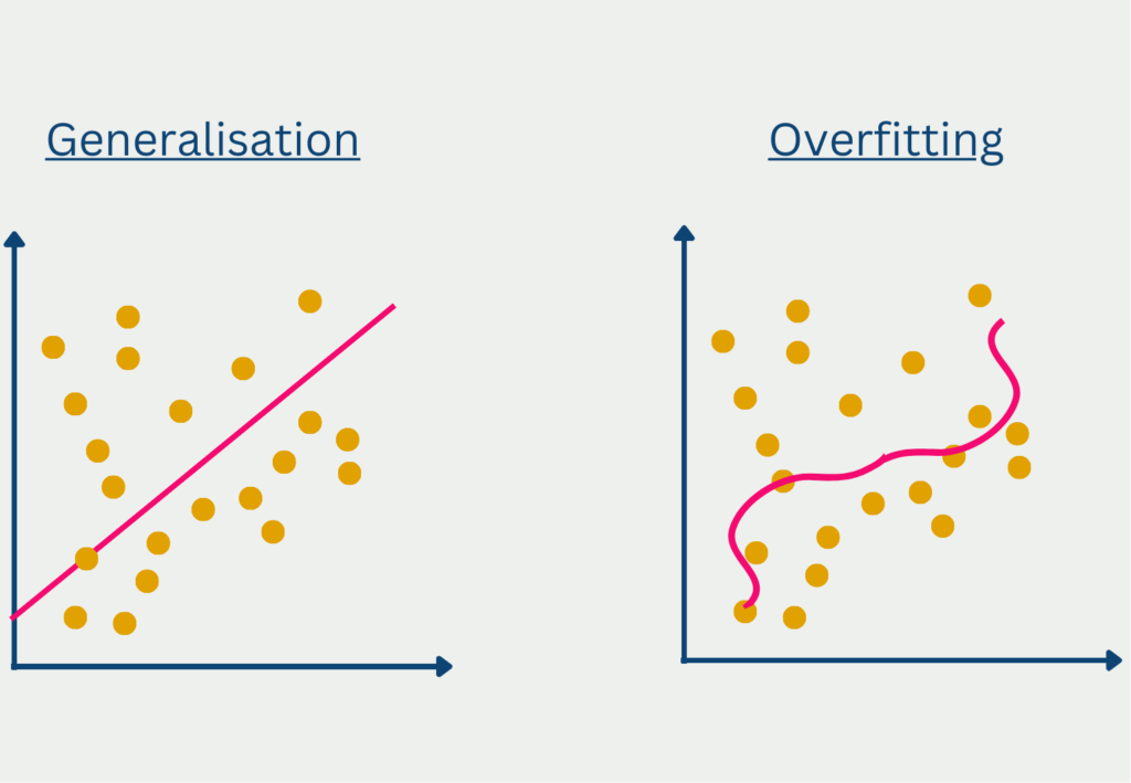
What is Overfitting?

Overfitting refers to the situation where a model has overfitted to the training data and does not generalize well to unseen data. This can be recognized by the fact that the results for predictions in the training data set are very good, but the model only achieves very low accuracies for new, unseen data.

In most cases, overfitting is caused by two things. If the model is too complex, i.e. contains too many parameters, then it has too many opportunities to learn the details of the training data set, which may not even occur outside the data set.
Overfitting can also occur if only a limited amount of data is available or the training dataset does not correspond to the general distribution as it occurs in reality. For example, if you want to train a model that is supposed to make predictions for the entire population of a country, overfitting is very likely to occur if you use a data set that only contains people under the age of 30.

Finally, another possible reason for overfitting can be an excessive number of training iterations. In each run, the model attempts to make an improvement, i.e. to make more correct predictions on the training data set compared to the previous run. At a certain point, this is only possible if it responds even more strongly to the characteristics of the training data set and adapts to them.

In general, there is no metric or analysis that can return with certainty whether a model is overfitting or not. However, there are some parameters and analyses that can indicate overfitting.

The loss function measures how often the model makes a correct prediction. For a good model that also generalizes well to unseen data, the loss function decreases in the training data set and (!) in the validation data set as the training data increases. This indicates that the model recognizes the underlying data structure and also provides good predictions for new data. With an overfitted model, on the other hand, the loss function in the validation data set decreases and starts to increase again at a certain point. This indicates that the model is now adapting too strongly to the training data and therefore the results for unseen data in the validation set are getting worse.

What is the Bias-Variance Tradeoff?

The bias-variance trade-off describes a fundamental problem in machine learning, which states that a compromise must be made between a model that is as simple as possible and a highly adaptable model that also delivers good results for new data.

The two central aspects of bias and variance are in conflict in every training. Before we can take a closer look at this problem, we should understand exactly what bias and variance are.

Bias describes the problem that a model that is too simple does not recognize the underlying structures in the data and therefore always predicts deviating values, leaving a certain residual error. However, you do not want to make the model too complex during training in order to prevent overfitting, which in turn would mean poor generalization to unseen data.

The variance, on the other hand, describes how strongly the predictions of a model fluctuate when the input values change only minimally. A high variance would mean that slight changes in the input would lead to very strong changes in the predictions.

A good machine learning model should have the lowest possible variance so that slight changes only have a minor impact on the predictions and the model therefore delivers reliable and robust predictions. At the same time, however, the bias should also be low, so that the prediction is as close as possible to the actual experience.

This results in a conflict of conscience, which is summarized as the bias variance tradeoff. In order to achieve a lower bias, the model must become more complex, which in turn leads to potential overfitting and a higher variance. Conversely, the variance can be reduced by reducing the complexity of the model, but this again leads to an increase in bias.

The trick now is to find a good compromise between an acceptable level of bias and an acceptable level of variance. It is important to understand this fundamental relationship in order to take it into account and integrate it into all areas of model training.

What types of regularization are there?

Regularization includes various techniques that aim to improve machine learning models by controlling model complexity and preventing overfitting. Over time, different types of regularization have developed with their own advantages and disadvantages, which we will present in more detail in this section.

L1 – Regularization (Lasso)

L1 regularization, or Lasso (Least Absolute Shrinkage and Selection Operator), aims to minimize the absolute sum of all network parameters. This means that the model is penalized if the size of the parameters increases too much. This procedure can result in individual model parameters being set to zero during L1 regularization, which means that certain features in the data set are no longer taken into account. This results in a smaller model with less complexity, which only includes the most important features for the prediction.

Mathematically speaking, another term is added to the cost function. In our example, we assume a loss function with a mean squared error, in which the average squared deviation between the actual value from the data set and the prediction is calculated. The smaller this deviation, the better the model is at making the most accurate predictions possible.

The following cost function then results for a model with the mean squared error as the loss function and an L1 regularization:

\(\) \[J\left(\theta\right)=\frac{1}{m}\sum_{i=1}^{m}\left(y_i-\widehat{y_i}\right)^2+\lambda\sum_{j=1}^{n}\left|\theta_j\right|\]

\(J\) is the cost function.
\(\lambda\) is the regularization parameter that determines how strongly the regularization influences the error of the model.
\(\sum_{j=1}^{n}\left|\theta_j\right|\) is the sum of all parameters of the model.

The aim of the model is to minimize this cost function. So if the sum of the parameters increases, the cost function increases and there is an incentive to counteract this. \(\lambda\) can assume any positive value (>= 0). A value close to 0 stands for a less strong regularization, while a large value stands for a strong regularization. With the help of cross-validation, for example, different models with different degrees of regularization can be tested to find the optimal balance depending on the data.

Advantages of L1 regularization:

Feature selection: Because the model is incentivized not to let the size of the parameters increase too much, a few of the parameters are also set to 0. This removes certain features from the data set and automatically selects the most important features.
Simplicity: A model with fewer features is easier to understand and interpret.

Disadvantages of L1 regularization:

Problems with correlated variables: If several variables in the data set are correlated with each other, Lasso tends to keep only one of the variables and set the other correlated variables to zero. This can result in information being lost that would have been present in the other variables.

L2 – Regularization (Ridge)

L2 regularization attempts to counter the problem of Lasso, i.e. the removal of variables that still contain information, by using the square of the parameters as the regularization term. Thus, it adds a penalty to the model that is proportional to the square of the parameters. As a result, the parameters do not go completely to zero, but merely become smaller. The closer a parameter gets to zero in mathematical terms, the smaller its squared influence on the cost function becomes. This is why the model concentrates on other parameters before completely eliminating a parameter close to zero.

Mathematically, the ridge regularization for a model with the mean squared error as the loss function looks as follows:

\(\)\[J\left(\theta\right)=\frac{1}{m}\sum{\left(i=1\right)^m\left(y_i-\widehat{y_i}\right)^2}+\lambda\sum_{j=1}^{n}{\theta_j^2}\]

The parameters here are identical to the previous formula with the difference that the absolute value theta is not summed up, but the square.

Advantages of L2 regularization:

Stabilization: Ridge regularization ensures that the parameters react much more stably to small changes in the training data.
Handling of multicollinearity: In the case of several correlated variables, L2 regularization ensures that these are considered together and not just one variable is kept in the model while the others are thrown out.

Disadvantages of L2 regularization:

No feature selection: Because Ridge does not set the parameters to zero, all features from the data set are retained in the model, which makes it less interpretable as more variables are taken into account.

Elastic Net

The Elastic Net tries to combine the best of both worlds by including both a term from the L1 regularization and a term from the L2 regularization in the cost function. This allows both feature selection to take place and multicollinear variables to be retained at the same time. The balance between the two regularizations can be set via the two parameters \(\lambda_1\) and \(\lambda_2\).

\(\)\[J\left(\theta\right)=\frac{1}{m}\sum_{i=1}^{m}\left(y_i-\widehat{y_i}\right)^2+\alpha\left(\lambda_1\sum_{j=1}^{n}\left|\theta_j\right|+\lambda_2\sum_{j=1}^{n}\theta_j^2\right)\]

The parameter \(\alpha\) determines the overall influence of the regularization on the cost function and \(\lambda_1\) and \(\lambda_2\) indicate the balance between the two methods.

How can Regularization be implemented in Python?

In Python, you can use the Scikit-Learn module to directly import regressions that already include the corresponding regularization methods. In this section, we will train a total of three models on random training data and compare the results in each case.

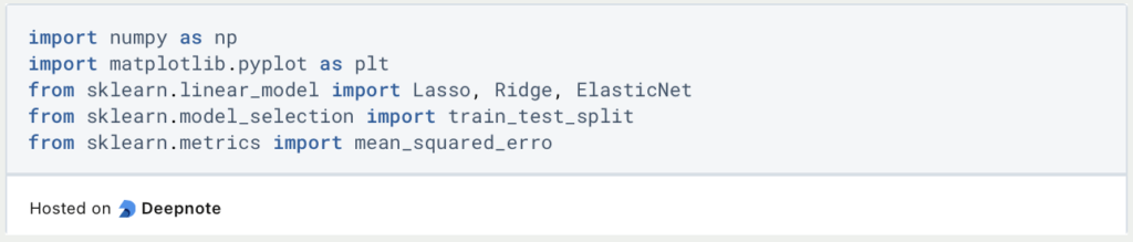
The first step is to import the necessary modules. In addition to Scikit-Learn, which we need for the models and their loss functions, we also import NumPy for generating the random training data and Matplotlib in order to be able to visualize the different results at the end.

To generate an exemplary training data set, we use NumPy and set np.random.seed(42) so that the same data is always generated when the program is run several times. We will have a total of 100 data points with five features each, which are created with np.random.rand. For each of the features, we define a parameter that the model should learn during training.

In order for these parameter values to be recognized and learned in the data set, we multiply our data point by the parameters, resulting in the target variable y. To ensure that the model does not have it too easy, we add noise, which is then added.

Finally, we split the data set into training and test data so that we can later compare the results of the models on new, unseen data.

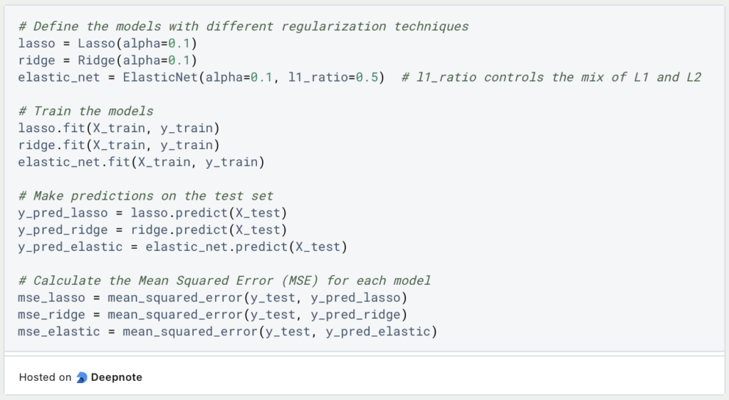
Now comes the exciting part where we create and train the individual models. For lasso and ridge, we only have to define the size of the regulation using the hyperparameter alpha. With ElasticNet, however, we also have to define the ratio between lasso and ridge. A good starting point for this is 0.5, whereby the two regularization methods are weighted equally.

We then train the individual models and let them make predictions for the test set. So that we can compare these results neutrally, we calculate the mean squared error for each combination of test set and prediction, which should already give a good picture of the performance of the different models.

These results are now output and we also look at the learned values of the parameters to see how close they came to the previously defined result.

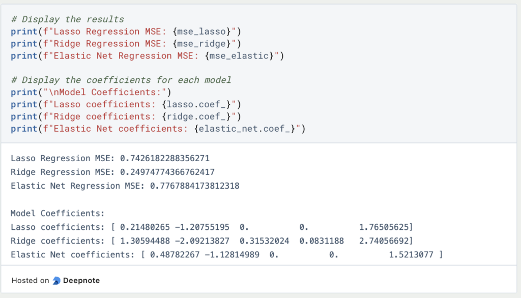
As we can see, as expected, only Lasso and Elastic Net were able to correctly predict parameters three and four, as Ridge is not able to set a parameter to zero. Overall, however, Ridge Regression performed best in this example, clearly beating the other two regularization methods.

The following diagram shows once again how the individual models estimated the parameters.

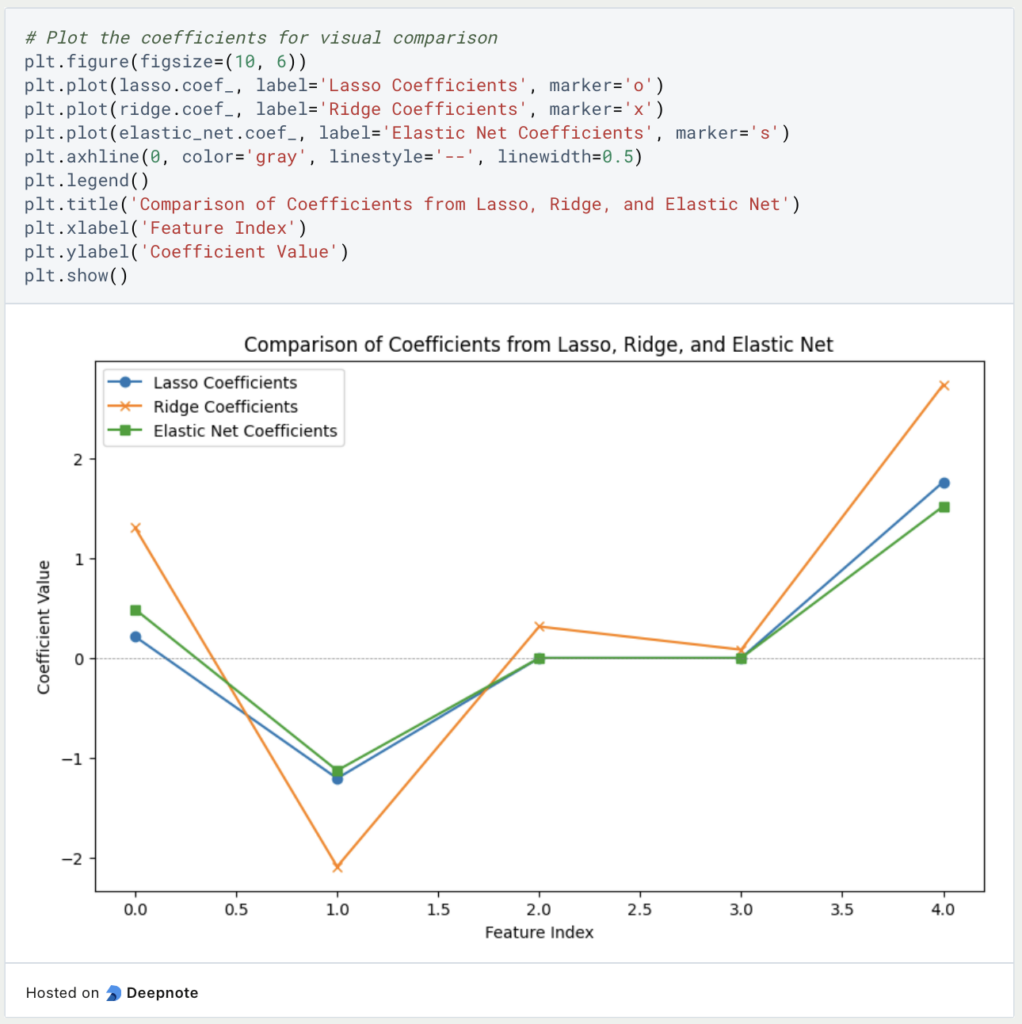
A possible starting point for ElasticNet would be to work with a different weighting between Ridge and Lasso again and to tend more towards Ridge. This could be used to test whether this change delivers better results.

What are advanced Regularization techniques?

The regularization techniques presented so far are particularly suitable for regressions and other classic machine learning models. However, methods have also been developed that work particularly well for deep learning and neural networks and which we present in more detail in this section.

Dropout Layer

In a neural network, the prediction is generated by running through different layers of neurons, each of which has its own weighting, which can change during training. The aim of the model is to minimize the loss function through these changes and thus make better predictions.

In a dropout layer, certain neurons are set to zero in a training run, i.e. removed from the network. This means that they have no influence on the prediction or backpropagation. As a result, a new, slightly modified network architecture is built in each run and the network learns to generate good predictions without certain inputs.

In deep neural networks, overfitting usually occurs when certain neurons from different layers influence each other. Simply put, this leads, for example, to certain neurons correcting the errors of previous nodes and thus depending on each other or simply passing on the good results of the previous layer without major changes. This results in poor generalization.

By using the dropout layer, on the other hand, the neurons can no longer rely on the nodes from previous or subsequent layers, as they cannot assume that these even exist in the respective training run. This leads to the neurons demonstrably recognizing more fundamental structures in data that do not depend on the existence of individual neurons. These dependencies actually occur frequently in regular neural networks, as this is an easy way to quickly reduce the loss function and thereby quickly get closer to the model’s goal.

Furthermore, as mentioned before, the dropout slightly changes the architecture of the network. Thus, the trained model is then a combination of many, slightly different models. We are already familiar with this approach from ensemble learning, for example in Random Forests. It turns out that the ensemble of many, relatively similar models usually delivers better results than a single model. This phenomenon is known as the “wisdom of the crowds”.

Data Augmentation

In many applications, especially in the field of supervised learning, the available data sets and their size are limited. At the same time, however, they are often too small to train complex models, resulting in overfitting. Data augmentation offers a way of artificially enlarging the data set by slightly modifying existing data points and adding them to the data set. In image processing, this can mean, for example, that an image appears in the data set once in color, once in black and white and once slightly rotated.

This approach not only increases the size of the data set, but the model also learns to generalize better, as there is greater variability in the training data and the risk of overfitting is reduced.

Early Stopping

When training deep learning models, the training runs through different epochs. In each epoch, each data point in the data set is fed into the network once. It is difficult to determine in advance how many epochs are required until the network has recognized and learned the basic structures. However, if the training takes too long, the model will continue to try to minimize the loss function. From a certain point onwards, however, this is only possible if the model adapts even more strongly to the training data, i.e. overfits.

In order to be able to wait for this point, which is not known before training, the early stopping rule is used, which automatically ends the training if the previously defined metric no longer improves over a certain period of epochs. In many cases, for example, the accuracy on the validation set is used, which is a special subset of the data set that is used after each epoch to determine how the model reacts to unseen data. If the accuracy on the validation set does not increase for several epochs, then the training stops automatically.

This is what you should take with you

Regularization includes methods in machine learning that are intended to limit overfitting and help deal with the bias-variance tradeoff.
An additional regularization term is added to the loss function.
A distinction is made between L1 regularization, also known as Lasso, L2 regularization, also known as Ridge, and Elastic Net.
In Python, these methods can be implemented directly using scikit-learn.
For neural networks, there are other ways to prevent overfitting, for example using dropout layers or an early stopping rule.

Thanks to Deepnote for sponsoring this article! Deepnote offers me the possibility to embed Python code easily and quickly on this website and also to host the related notebooks in the cloud.