Dimensionality reduction is a central method in the field of Data Analysis and Machine Learning that makes it possible to reduce the number of dimensions in a data set while retaining as much of the information it contains as possible. This step is necessary to reduce the dimensionality of the data set before training in order to save computing power and avoid the problem of overfitting.

In this article, we take a detailed look at dimensionality reduction and its objectives. We also illustrate the most commonly used methods and highlight the challenges of dimensionality reduction.

What is Dimensionality Reduction?

Dimensionality reduction comprises various methods that aim to reduce the number of characteristics and variables in a data set while preserving the information in the data set. In other words, fewer dimensions should enable a simplified representation of the data without losing patterns and structures within the data. This can significantly accelerate downstream analyses and also optimize machine learning models.

In many applications, problems occur due to the high number of variables in a data set, which is also referred to as the curse of dimensionality, which we will discuss in more detail in the following section. For example, too much dimensionality can lead to these problems:

• Overfitting: When machine learning models become overly reliant on characteristics of the training dataset and therefore only provide poor results for new, unseen data, this is known as overfitting. With a high number of features, the risk of overfitting increases as the model becomes more complex and therefore adapts too strongly to the errors in the data set.
• Computational complexity: Analyses and models that have to process many variables often require more parameters to be trained. This increases the computational complexity, which is reflected either in a longer training time or in increased resource consumption.
• Data Noise: With an increased number of variables, the probability of erroneous data or so-called noise also increases. This can influence the analyses and lead to incorrect predictions.

Although large data sets with many characteristics are very informative and valuable, the high number of dimensions can also quickly lead to problems. Dimensionality reduction is a method that attempts to preserve the information content of the data set while reducing the number of dimensions.

What is the Curse of Dimensionality?

The Curse of Dimensionality occurs with high-dimensional data sets, i.e. those that have a large number of attributes or features. At first, many attributes are a good thing because they contain a lot of information and describe the data points well. For example, if we have a dataset about people, the attributes can be information such as hair color, height, weight, eye color, etc.

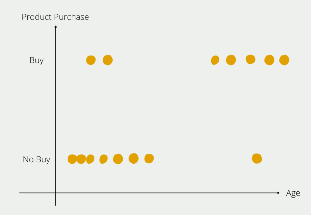
In mathematical terms, however, each additional attribute means a new dimension in the space and therefore a significant increase in possibilities. This becomes clear from the following example, in which we want to find out which customers buy which products. In the first step, we only look at the age of the prospective customers and whether they have bought the product. We can still depict this relatively easily in a two-dimensional diagram.

As soon as we add more information about the customer, things get a little more complex. The information on the customer’s income would mean a new axis on which the numerical income is mapped. So the two-dimensional diagram becomes a three-dimensional one. The additional attribute “gender” would lead to a fourth dimension and so on.

When working with data, it is desirable to have a lot of attributes and information in the data set in order to give the model many opportunities to recognize structures in the data. However, it can also lead to serious problems, as the name Curse of Dimensionality suggests.

Data Sparsity

The example shown illustrates a problem that occurs with many attributes. Due to the large number of dimensions, the so-called data space, i.e. the number of values that a data set can take on, also grows. This can lead to what is known as data sparsity. This means that the training data set used to train the model does not contain certain values at all or only very rarely. As a result, the model only delivers poor results for these marginal cases.

Let’s assume that we examine 1,000 customers in our example, as it would be too time-consuming to survey even more customers or this data is simply not available. It is possible that all age groups from young to old are well represented among these customers. However, if the additional dimension of income is added, it becomes less likely that the possible characteristics, such as “young” and “high income” or “old” and “medium income”, will occur and be backed up with enough data points.

Distance Concentration

If you want to evaluate the similarity of different data sets in the field of machine learning, distance functions are often used for this. The most common clustering algorithms, such as k-means clustering, rely on calculating the distance between points and assigning them to a cluster depending on their size. In multidimensional spaces, however, it can quickly become the case that all points are at a similar distance from each other, so that it seems almost impossible to separate them.

We are also familiar with this phenomenon from everyday life. If you take a photo of two objects, such as two trees, they can look very close to each other in the picture, as it is only a two-dimensional image. In real life, however, the trees may be several meters apart, which only becomes clear in three dimensions.

These problems, which can occur in connection with many dimensions, are summarized under the term Curse of Dimensionality.

What are the Goals of Dimensionality Reduction?

Dimensionality reduction primarily pursues three primary goals: Improving model performance, visualizing data and increasing processing speed. We will examine these in more detail in the following section.

Improving Model Performance

One of the main goals of dimensionality reduction is to improve model performance. By reducing the number of variables in a dataset, a less complex model can be used, which in turn reduces the risk of overfitting.

Models that have a large number of parameters and are therefore highly complex tend to overfit to the training dataset and the noise in the data. As a result, the model delivers poorer results with new data that does not contain this noise, while the accuracy of the training data set is very good. This phenomenon is known as overfitting. During dimensionality reduction, unimportant or redundant features are removed from the data set, which reduces the risk of overfitting. As a result, the model delivers better quality for new, unseen data.

Visualization of Data

If you want to visualize data sets with many features, you face the challenge of mapping all this information in a two- or at most three-dimensional space. Any dimensionality beyond this is no longer directly tangible for us humans, but it is easiest to assign a separate dimension to each feature in the data set. Therefore, with high-dimensional data sets, we are often faced with the problem that we cannot simply visualize the data in order to gain an initial understanding of the peculiarities of the data and, for example, to recognize whether there are outliers.

Dimensionality reduction helps to reduce the number of dimensions to such an extent that visualization in two- or three-dimensional space is possible. This makes it easier to better understand the relationships between the variables and the data structures.

Increasing the Processing Speed

Computing time and the necessary resources play a major role in the implementation of projects, especially for machine learning and deep learning algorithms. Often, only limited resources are available, which should be used optimally. By removing redundant features from the data set at an early stage, you not only save time and computing power during data preparation, but also when training the model, without having to accept lower performance.

In addition, dimensionality reduction makes it possible to use simpler models that not only require less power during initial training, but can also perform calculations faster later during operation. This is an important factor, especially for real-time calculations.

Overall, dimensionality reduction is an important method for improving data analysis and building more robust machine learning models. It is also an important step in the visualization of data.

Which Methods are used for Dimensionality Reduction?

In practice, various methods for dimensionality reduction have become established, three of which are explained in more detail below. Depending on the application and the structure of the data, these methods already cover a broad spectrum and can be used for most practical problems.

Principal Component Analysis

Principal component analysis (PCA) assumes that several variables in a data set possibly measure the same thing, i.e. are correlated. These different dimensions can be mathematically combined into so-called principal components without compromising the significance of the data set. Shoe size and height, for example, are often correlated and can therefore be replaced by a common dimension to reduce the number of input variables.

Principal component analysis describes a method for mathematically calculating these components. The following two key concepts are central to this:

The covariance matrix is a matrix that specifies the pairwise covariances between two different dimensions of the data space. It is a square matrix, i.e. it has as many rows as columns. For any two dimensions, the covariance is calculated as follows:

\(\)\[ \text{Cov}\left(X, Y\right) = \frac{\sum_{i=1}^{n}\left(X_i – \bar{X}\right)\cdot\left(Y_i – \bar{Y}\right)}{n – 1} \]

Here \(n\) stands for the number of data points in the data set, \(X_i\) is the value of the dimension \(X\) of the ith data point and \(\bar{X}\) is the mean value of the dimension \(X\) for all \(n\) data points. As can be seen from the formula, the covariances between two dimensions do not depend on the order of the dimensions, so the following applies \(COV(X,Y) = COV(Y,X)\). These values result in the following covariance matrix \(C\) for the two dimensions \(X\) and \(Y\):

\(\) \[C=\left[\begin{matrix}Cov(X,X)&Cov(X,Y)\\Cov(Y,X)&Cov(Y,Y)\\\end{matrix}\right]\]

The covariance of two identical dimensions is simply the variance of the dimension itself, i.e:

\(\)\[C=\left[\begin{matrix}Var(X)&Cov(X,Y)\\Cov(Y,X)&Var(Y)\\\end{matrix}\right]\]

The covariance matrix is the first important step in the principal component analysis. Once this matrix has been created, the eigenvalues and eigenvectors can be calculated from it. Mathematically, the following equation is solved for the eigenvalues:

\(\)\[\det{\left(C-\ \lambda I\right)}=0\]

Here \(\lambda\) is the desired eigenvalue and \(I\) is the unit matrix of the same size as the covariance matrix \(C\). When this equation is solved, one or more eigenvalues of a matrix are obtained. They represent the linear transformation of the matrix in the direction of the associated eigenvector. An associated eigenvector can therefore also be calculated for each eigenvalue, for which the slightly modified equation must be solved:

\(\) \[\left(A-\ \lambda I\right)\cdot v=0\]

Where \(v\) is the desired eigenvector, according to which the equation must be solved accordingly. In the case of the covariance matrix, the eigenvalue corresponds to the variance of the eigenvector, which in turn represents a principal component. Each eigenvector is therefore a mixture of different dimensions of the data set, the principal components. The corresponding eigenvalue therefore indicates how much variance of the data set is explained by the eigenvector. The higher this value, the more important the principal component is, as it contains a large proportion of the information in the data set.

Therefore, after calculating the eigenvalues, they are sorted by size and the eigenvalues with the highest values are selected. The corresponding eigenvectors are then calculated and used as principal components. This results in a reduction in dimension, as only the principal components are used to train the model instead of the individual features of the data set.

t-Distributed Stochastic Neighbor Embedding (t-SNE)

t-Distributed Stochastic Neighbor Embedding, or t-SNE for short, approaches the problem of dimensionality reduction differently by attempting to create a new, lower-dimensional space that adopts the distances of the data points from the higher-dimensional space as far as possible. The basic idea of this becomes clear in the following example.

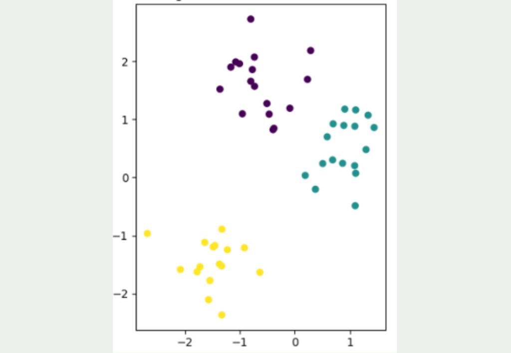
It is not easy to transfer data sets from a high dimensionality to a low dimensionality while retaining as much information as possible from the data set. The following figure shows a simple, two-dimensional data set with a total of 50 data points. Three different clusters can be clearly identified, which are also well separated from each other. The yellow cluster is furthest away from the other two clusters, while the purple and blue data points are closer to each other.

The aim now is to convert this two-dimensional data set into a lower dimension, i.e. into one dimension. The simplest approach for this would be to represent the data either only by its X or Y coordinate.

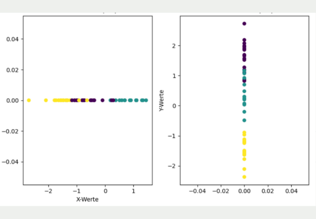
However, it is clear that this simple transformation has lost much of the information in the data set and gives a different picture than the original two-dimensional data. If only the X coordinates are used, it looks as if the yellow and purple clusters overlap and that all three clusters are roughly equidistant from each other. If, on the other hand, only the Y coordinates are used for dimensionality reduction, the yellow cluster is much better separated from the other clusters, but it looks as if the purple and blue clusters overlap.

The basic idea of t-SNE is that the distances from the high dimensionality are transferred to the low dimensionality as far as possible. To do this, it uses a stochastic approach and converts the distances between points into a probability that indicates how likely it is that two random points are next to each other.

More precisely, it is a conditional probability that indicates how likely it is that one point would choose the other point as a neighbor. Hence the name “Stochastic Neighbor Embedding”.

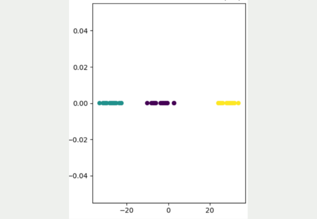
As you can see, this approach leads to a much better result, in which the three different clusters can be clearly distinguished from one another. It is also clear that the yellow data points are significantly further away from the other data points and the blue and purple clusters are somewhat closer together. To better understand the details of this approach, you are welcome to read our detailed article on this topic.

Linear Discriminant Analysis

Linear Discriminant Analysis (LDA for short) aims to identify and maximize the separability between classes by projecting the data onto a smaller dimension. In contrast to other methods, it places particular emphasis on maximizing the separability between classes and is therefore particularly important for classification tasks.

Two central key figures are calculated:

• Within-Class Scatter: This key figure measures the variability within a class of data. The lower this value, the more similar the data points are within a class and the more clearly the classes are separated.
• Between-class scatter: This scatter in turn measures the variability between the mean values of the classes. This value should be as large as possible, as this indicates that the classes are easier to separate from each other.

Simply put, these key figures are used to form matrices and calculate their eigenvalues. The eigenvectors for the largest eigenvalues are in turn the dimensions in the new feature space, which has fewer dimensions than the original data set. All data points can then be projected onto the eigenvectors, which reduces the dimensions.

Linear Discriminant Analysis is particularly suitable for applications in which the classes are already known and the data is also clearly labeled. It uses this class information from supervised learning to find a low-dimensional space that separates the classes as well as possible.

A disadvantage of LDA is that the maximum reduction to a dimensional space is limited and depends on the number of classes. A data set with \(n\) classes can therefore be reduced to a maximum of \(n-1\) dimensions. In concrete terms, this means, for example, that a data set with three different classes can be reduced to a two-dimensional space.

This approach of dimensionality reduction is also particularly suitable for large data sets, as the computing effort is only moderate and scales well with the amount of data, so that the computing effort is kept within limits even with large amounts of data.

What are the Challenges of Dimensionality Reduction?

Dimensionality reduction is an important step in data pre-processing in order to increase the generalizability of machine learning models and the general model performance and possibly save computing power. However, the methods also bring with them some challenges that should be considered before use. These include

• Loss of information: Although the methods presented attempt to retain as much variance, i.e. information content, of the data set, some information is inevitably lost when dimensions are reduced. Important data can also be lost, which may lead to poorer analyses or model results. Therefore, the resulting model may be less accurate or less powerful.
• Interpretability: Most algorithms used for dimensionality reduction provide a low-dimensional space that no longer contains the original dimensions, but a mathematical summary of them. Principal component analysis, for example, uses the eigenvectors, which are a summary of various dimensions from the data set. As a result, interpretability is lost to a certain extent, as the previous dimensions are easier to measure and visualize. Especially in use cases where transparency is important and the results require a practical interpretation, this can be a decisive disadvantage.
• Scaling: Performing dimensionality reductions is computationally intensive and takes time, especially for large data sets. In real-time applications, however, this time is not available, as the computing time of the model is added to this. Computing-intensive models in particular, such as t-SNE or autoencoders, quickly fall out because they take too long to make live predictions.
• Selecting the method: Depending on the application, the dimensionality reduction methods presented have their strengths and weaknesses. The selection of a suitable algorithm therefore plays an important role, as it has a significant influence on the results. There is no one-size-fits-all solution and a new decision must always be made based on the application.

Dimensionality reduction has many advantages and is an integral part of data pre-processing in many applications. However, the disadvantages and challenges mentioned must also be taken into account in order to train an efficient model.

This is what you should take with you

• Dimensionality reduction is a method of reducing the number of dimensions, i.e. variables, in a data set while retaining as much information content as possible.
• With many input variables, the so-called curse of dimensionality arises. This leads to problems such as data sparsity or distance concentration.
• Dimensionality reduction often leads to a lower probability of overfitting, better visualization and optimized computing power when training machine learning models.
• The most common dimensionality reduction methods include principal component analysis, t-SNE and LDA.
• However, dimensionality reduction also has disadvantages, such as poorer interpretability or loss of information.

Other Articles on the Topic of Dimensionality Reduction

You can find practical examples of how to do dimensionality reduction in Scikit-Learn here.