If robust machine learning models are to be trained, large data sets with many dimensions are required to recognize sufficient structures and deliver the best possible predictions. However, such high-dimensional data is difficult to visualize and understand. This is why dimension reduction methods are needed to visualize complex data structures and perform an analysis.

The t-Distributed Stochastic Neighbor Embedding (t-SNE/tSNE) is a dimension reduction method that is based on distances between the data points and attempts to maintain these distances in lower dimensions. It is a method from the field of unsupervised learning and is also able to separate non-linear data, i.e. data that cannot be divided by a line.

Why is dimension reduction needed?

Various algorithms, such as linear regression, have problems if the data set contains variables that are correlated, i.e. dependent on each other. To avoid this problem, it can make sense to remove the variables from the data set that correlate with another variable. At the same time, however, the data should not lose its original information content or should retain as much information as possible.

Another application is cluster analysis, such as k-means clustering, where we have to define the number of clusters in advance. Reducing the dimensionality of the data set helps us to get a first impression of the information and, for example, to be able to estimate which are the most important variables and how many clusters the data set could have. For example, if we manage to reduce the data set to three dimensions, we can visualize the data points in a diagram. The number of clusters can then possibly be read from this.

In addition, large data sets with many variables also pose the risk of the model overfitting. In simple terms, this means that the model adapts too much to the training data during training and therefore only delivers poor results for new, unseen data. For neural networks, for example, it can therefore make sense to first train the model with the most important variables and then gradually add new variables that may further increase the performance of the model without overfitting.

What are the basic principles of t-SNE?

t-Distributed Stochastic Neighbor Embedding is based on several fundamental concepts, which are explained in more detail below to help you understand the basic features of the algorithm:

Similarity measure: The similarity between data points is visualized using distance measures that measure how far apart two points are. The Euclidean distance is typically used for this, where the difference between the coordinates of two points is formed in all dimensions. These differences are then squared and added together. In addition to calculating the distance, other similarity measures can also be used, such as cosine similarity. The angle between two vectors determines how similar they are. The smaller the included angle, the more similar the data points.

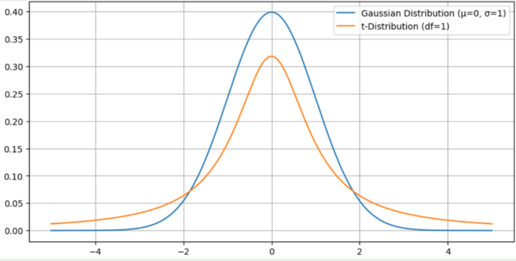
Probability distribution: The t-SNE uses two probability distributions. In high-dimensional space, an attempt is made to place all data points on a Gaussian normal distribution. A data point is positioned in the center of the bell curve and the remaining points of the data set are placed on the Gaussian normal distribution based on their distance from this point. The closer a point is to the selected data point, the closer this point is to the center of the bell curve.

In low-dimensional space, on the other hand, the t-distribution is used, which is similar to the normal distribution with the difference that the edges are slightly higher and therefore the center is slightly lower. The t-SNE algorithm aims to find a way of converting the Gaussian distribution in high-dimensional space into a t-distribution in low-dimensional space while losing as little information as possible.

• Embedding function: To complete the algorithm, an embedding function is created that enables data points in high-dimensional space to be mapped to points in low-dimensional space. Each point in the high-dimensional space is assigned exactly one point in the low-dimensional space.

These basic principles form the basis for a good understanding of the t-SNE algorithm.

What is the idea behind t-SNE?

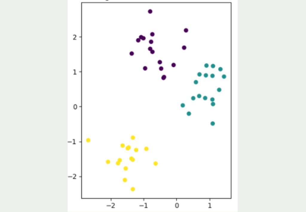
It is not easy to convert data sets from a high dimensionality to a low dimensionality while retaining as much information as possible from the data set. The following figure shows a simple, two-dimensional data set with a total of 50 data points. Three different clusters can be identified, which are also well separated from each other. The yellow cluster is furthest away from the other two clusters, while the purple and blue data points are closer to each other.

The aim now is to convert this two-dimensional data set into a lower dimension, i.e. into one dimension. The simplest approach for this would be to represent the data either only by its X or Y coordinate.

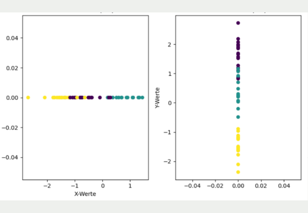
However, it is clear that this simple transformation has lost much of the information in the data set and gives a different picture than the original two-dimensional data.

If only the X coordinates are used, it looks as if the yellow and purple clusters overlap and that all three clusters are roughly equidistant from each other. If, on the other hand, only the Y coordinates are used for dimensionality reduction, the yellow cluster is much better separated from the other clusters, but it looks as if the purple and blue clusters overlap.

The basic idea of t-SNE is that the distances from the high dimensionality are transferred to the low dimensionality as far as possible. To do this, it uses a stochastic approach and converts the distances between the points into a probability that indicates how likely it is that two random points are next to each other.

More precisely, it is a conditional probability that indicates how likely it is that one point would choose the other point as a neighbor. Hence the name “Stochastic Neighbor Embedding”.

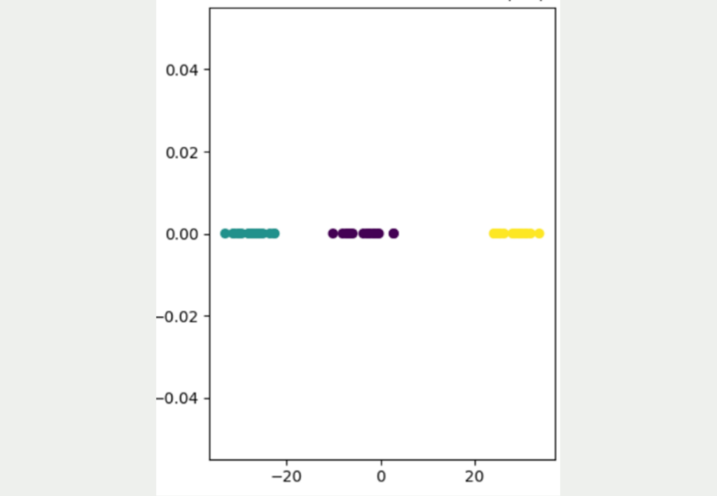
As you can see, this approach leads to a much better result, in which the three different clusters can be clearly distinguished from one another. It is also clear that the yellow data points are significantly further away from the other data points and that the blue and purple clusters are somewhat closer together.

How does the t-SNE algorithm work?

In the first step, the t-SNE algorithm calculates a Gaussian probability distribution for all points. This indicates how likely it is that two randomly selected points are neighbors. A high probability indicates that the two points are close to each other, while a low probability indicates a large distance between the points.

For any given yellow data point, this distribution might look like the diagram below. The other yellow data points are very close to the selected point and therefore have a high probability of being a neighbor of the selected point. The blue and purple points have partially similar distances and therefore overlap. However, they are all significantly less likely to be a neighbor and are therefore further out on the normal distribution.

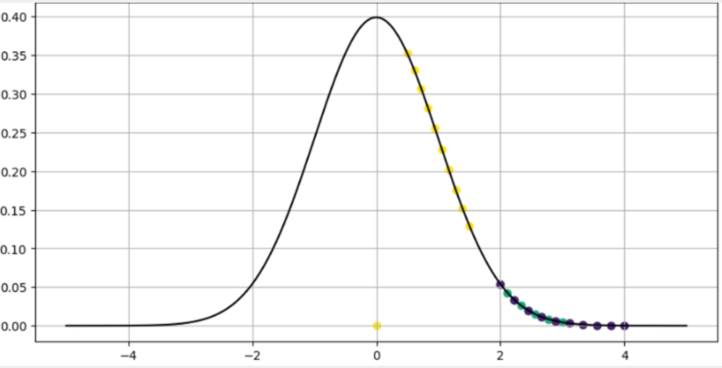
The paper in which t-SNE was first described also states that the conditional probability of a point to itself is defined as zero. Therefore, a data point lies at the origin of the graph, as this point cannot be the neighbor to itself.

Mathematically, this curve is expressed as the conditional probability that two points \( x_j \) and \(x_i \) are adjacent to each other. This is the first part of t-SNE, namely the “Stochastic Neighbor Embedding”, whereby the neighborhood of two points can be expressed using probabilities. This probability can be calculated using the formula 

\(\) \[
p_{(j|i)} = \frac{\exp \left( – \frac{ \left\| x_i – x_j \right\|^2 }{ 2 \sigma_i^2 } \right)}{\sum_{k \neq l} \exp \left( – \frac{ \left\| x_k – x_l \right\|^2 }{ 2 \sigma_i^2 } \right)}
\]

The individual parameters mean in detail:

• \( p_{(j|i)}\): This represents the probability that the point \(x_i \)would choose the point \( x_j \) as its direct neighbor in high-dimensional space.
•  \(x_i\) and \(x_j\) are the two data points in high-dimensional space.
• \(\left\| x_i – x_j \right\| \) is the distance between the two points. The Euclidean distance is often used for this, but any desired distance metric can be used.
• \( \exp \left( – \frac{ \left\| x_i – x_j \right\|^2 }{ 2 \sigma_i^2 } \right) \) is the most complex part of this formula and is known as the Gaussian kernel function. This ensures the bell shape of the curve and, above all, causes distances to become probabilities between 0 and 1. Otherwise, the values of the distances would always depend on the scale in which the data set is located. The standard deviation of the point \( x_i \) depends on the so-called perplexity, which determines whether the model should focus more on the correct mapping of nearby points or distances between distant points. This parameter will be discussed in more detail in the next section.
• \( \sum_{k \neq l} \exp \left( – \frac{ \left\| x_k – x_l \right\|^2 }{ 2 \sigma_i^2 } \right) \) represents the sum of all conditional probabilities between the point \( x_l \) and all other data points in the dataset plus the point \( x_l \) itself. It is divided by this term to ensure that the sum of all conditional probabilities between the point \( x_i \) and all other data points in the dataset sums to one. Without this normalization term, the distribution would look like the previous diagram. The problem here, however, is that the sum of the probabilities of all data points is greater than 1. This characteristic ensures that an interpretable probability distribution is obtained.

After this conditional probability has been adapted to the high-dimensional data space, an attempt is then made to transfer it to a low-dimensional data space so that the conditional probabilities remain as similar as possible. With conventional “Student Neighbor Embedding”, an attempt would now be made to convert the conditional probability into a Gaussian distribution with new points in the low-dimensional space that fits as closely as possible. However, the “t” in t-SNE stands for the so-called student t-distribution, which has already been mentioned in the section on basic principles.

The t-distribution is characterized by the fact that it still assigns a comparatively high probability to points that are far from the mean compared to the Gaussian normal distribution. This property of the “heavy tails” makes it possible to sufficiently distinguish points in low-dimensional space that are far away from the analyzed point.

This property was described in stochastic neighbor embedding as the so-called crowding problem. It describes the case where points in low-dimensional space are too close to each other, especially if they are very far away from the analyzed point in high-dimensional space. This problem is solved by the t-distribution and its “heavy tails”, as it enables a certain degree of separation to be maintained even for points that are far away.

The so-called degrees of freedom in the t-distribution is a parameter that determines how many independent samples are used to create an estimate. These degrees of freedom also have a considerable influence on the distribution, as they indicate the extent to which the distribution is broadened. The more degrees of freedom, the narrower the distribution and the more it resembles the normal distribution.

A degree of freedom of one is selected for t-SNE to generate the “heavy tails” and thus have more measures outside the center, i.e. the mean value. Low degrees of freedom therefore mean a greater probability of outlier data. With t-SNE, this property is desirable to simulate the point-to-point relationships in low-dimensional space. This allows a balance to be established between the modeling of nearby and distant points.

Thus, the conditional probability from the high-dimensional space must be transferred to a t-distribution in the low-dimensional space. This is calculated using the following formula:

\(\) \[
q_{j|i} = \frac{(1 + \left\| y_i – y_j \right\|^2)^{-1}}{\sum_{k \neq l} (1 + \left\| y_k – y_l \right\|^2)^{-1}}
\]

These are:

• \(y_i \) and \(y_j \) are two data points in the low-dimensional space that represent the points from the high-dimensional space.
• \( q_{j|i} \) is the conditional probability that the points \( y_i \) and \( y_j \) are close to each other, i.e. are neighbors.
• \( \left\| y_i – y_j \right\| \) is the distance between the two points. The same distance metric should be selected here as in high-dimensional space, i.e. in most cases the Euclidean distance.
• \( (1 + \left\| y_i – y_j \right\|^2)^{-1} \) represents the similarity between two points in low-dimensional space. The t-distribution with one degree of freedom is used for this.
• \( \sum_{k \neq l} (1 + \left\| y_k – y_l \right\|^2)^{-1} \) is the sum of all probabilities between two different points in the data set. This sum is divided to bring about normalization and ensure that the probabilities add up to one.

The question now arises as to how the existing conditional probability in high-dimensional space can be transferred as effectively as possible to the conditional probability in low-dimensional space. For this purpose, an optimization problem is defined that uses the so-called Kullback-Leibler (KL) divergence. The gradient method is used to minimize the divergence between the high-dimensional and low-dimensional probabilities.

This article does not go into the mathematical formulation of this problem but merely describes the schematic procedure. The optimization is an iterative process in which the divergence of the two probabilities is calculated and then the derivative is calculated for a single point. This value indicates how much the low-dimensional mapping of a point should be changed. The sign determines the direction and the value of the strength of the change of a point. This allows the divergence between the two probabilities to be reduced and t-SNE aims to achieve the lowest possible divergence, as the conditional probability in high-dimensional and low-dimensional space is then as similar as possible.

This iterative process takes place until a so-called convergence criterion is reached, for example, a maximum number of repetitions has been reached or the divergence between the two probabilities has fallen below the specified value.

What are the hyperparameters of t-SNE?

The t-SNE algorithm has several hyperparameters that influence both the behavior and the performance of the model. This section introduces the key hyperparameters and shows how the model changes when these values are adjusted.

Perplexity measures how many neighbors are considered at each point during the embedding process. A high value means that more neighbors are included and therefore the distances of distant points are better mapped in the low dimensions. With a low perplexity, on the other hand, the focus is more on mapping the immediate proximity of the points as accurately as possible, even if the distant points are mapped less accurately.

The learning rate is the central hyperparameter for the gradient method, which changes the embedding positions in stepwise iterations so that the divergence between the two probability distributions is as small as possible. The learning rate determines the step size of the individual embedding updates.

With a high learning rate, large changes to the embeddings can take place in one iteration, which on the one hand can lead to faster convergence, but on the other hand can also lead to an unstable learning process, as the optimal result may be skipped and the model therefore fluctuates a lot. A low learning rate, on the other hand, means that more iterations will probably be needed to reach the optimum, but the training will be more uniform.

Before you can start the training, you must determine when the training should be stopped. To do this, either a threshold value for the divergence can be set, which leads to a stop as soon as it is undercut for the first time, or a maximum number of iterations can be set. This number determines how often the embedding positions can be optimized and can be in the hundreds or thousands for many applications.

The number of iterations should depend on the learning rate, the data, and the amount of resources available. If possible, it is best to use a combination and define a so-called early stopping rule in which the model either stops when the divergence threshold is reached or the maximum number of iterations is reached.

T-SNE aims to transform a high-dimensional data set in such a way that it manages with significantly fewer dimensions. The aim here is usually to limit the dimensions of the embedding space to two or three so that the data can be visualized and interpreted by human users. In this case, it makes sense to use three-dimensional embedding to give the model even more possibilities to depict the original information of the data set. A two-dimensional arrangement is often easier to interpret but also offers less information content.

Another hyperparameter when working with t-SNE is the distance measure that is used. By default, the Euclidean distance is selected, which squares the differences between all dimensions of two points and then adds them up. This metric is not only easy to calculate but is also a suitable starting point for many applications. In special cases, however, the choice of other distance metrics can be useful. These are, for example:

• Cosine distance: The so-called cosine similarity measures how similar two vectors are by determining the angle that the two vectors make to each other. The cosine distance is calculated by subtracting the cosine similarity from 1. The greater this distance, the more different the two vectors are. This metric is useful in natural language processing, for example, where words are represented by vectors. The similarity of the vectors, i.e. the meaning of the words used, is more important than the length of the vectors, which encodes the semantic meaning of the words.
• Manhattan distance: This distance metric is also known as the city block distance, as it does not calculate the direct distance between points, but the absolute difference in all dimensions. The nickname comes from the fact that it behaves like a cab driver in Manhattan who has to follow the streets and therefore drives from block to block. This distance metric should be used if the features in the dimensions are not normally distributed or if there are outliers in the data set.

These are the most important hyperparameters when training t-SNE. As with other models, there is no optimal setting for these values that is suitable for all applications and data sets. Rather, it is necessary to experiment with the hyperparameters to find the optimal set of values and train an efficient model.

What are the limitations of t-SNE?

t-SNE is a powerful way to reduce the dimensionality of datasets while retaining as much information as possible from the original data. However, some negative aspects should be considered before using it.

Performing t-SNE can be very computationally intensive and time-consuming, especially with large data sets. The optimization of the loss functions in particular requires many iterations until a meaningful result is obtained.

The algorithm uses several hyperparameters that have a major influence on the performance of the model and must therefore be set carefully. The selection of suitable values often requires various tests that take time and computing resources.

The loss function in t-SNE has the mathematical property that it is not convex. This means that the graph has several so-called local minima and only one unique, global minimum. A local minimum is characterized by the fact that it is the lowest point in a certain range, but not the absolute lowest point of the graph in the complete definition range. During the optimization of the loss function, an attempt is made to achieve a state in which the divergence between the probability distributions is as small as possible.

Depending on the size of the learning rate, it can now happen that the algorithm reaches a local minimum and does not move away from it, as the loss only increases in all possible steps of the learning rate. This fools the algorithm into believing that it is in an optimal state in which the loss is minimal. However, this is not the best possible configuration, but merely a local minimum.

Another disadvantage of t-SNE is that the algorithm does not learn a general embedding function that can also be applied to new data points. The probability distribution is only valid for the current data set and cannot be generalized to new points. Therefore, if the data set is enlarged, a new probability distribution must be calculated.

In addition, t-SNE is non-deterministic, so that several training runs with the same hyperparameters can lead to different results. This is related to the use of probability distributions. Several runs will lead to similar, but usually not identical, results.

Another important disadvantage of t-SNE is that global structures and distances are often lost and the focus is mainly on local structures. As a result, the global relationships can be misinterpreted, which is why t-SNE should only be used as a visualization aid for high-dimensional data and not for clustering data, as it can lead to incorrect results. It is also often misleading that the data appears to form perfect clusters after the application of t-SNE, although this is not necessarily the case in reality and is usually because the global structures are not optimally mapped and the focus is on the direct neighbors. 

t-SNE vs. PCA

t-SNE and PCA are two key dimension reduction techniques that are widely used in various analyses to reduce dimensionality and visualize high-dimensional data. However, there are some fundamental differences between the two methods that should be taken into account when choosing.

PCA is a linear dimensionality reduction method that is based on the covariance matrix and uses its eigenvalues and eigenvectors to find a low-dimensional representation of the data set. The eigenvectors with the highest eigenvalues are used to transfer the data into a data space and still obtain the maximum variance of the data set.

t-SNE, on the other hand, is a non-linear approach that aims to map the distances between data in a low-dimensional space as accurately as possible. For this purpose, the conditional probabilities that any two points are neighbors are calculated. A similar probability is then to be produced in the low-dimensional space. For this purpose, the Kullback-Leibler divergence between the two distributions is minimized step by step.

These different architectures also result in some differences:

• Linearity: As described, PCA is a linear methodology, meaning that only linear relationships between the data points can be recorded. This may often not be sufficient to capture the complexity of the data set. In contrast, t-SNE is a non-linear method that can also capture more complex relationships between the data.
• Interpretability: Principal component analysis often provides better interpretability, as the individual components are a linear summary of the original characteristics and it is also possible to determine which characteristic contributes to the principal components and to what extent. With t-SNE, on the other hand, the lower dimensions have no direct meaning with the original dimensions and are not so easy to interpret. Therefore, further analyses are often required to understand the actual meaning of the low dimensions.
• Computing time: Especially for large data sets with many dimensions, it is important how well the method can be scaled and how much computing time it takes. PCA often performs better than t-SNE, as it is a linear method, and therefore more efficient methods can be used. The computing time of t-SNE, on the other hand, is much more complicated to predict, as it is a complex, iterative optimization where it is difficult to predict the time until the result converges. If the data sets become larger, the computing time also increases accordingly, as iterative methods, such as the gradient method, become significantly more complex.
• Hyperparameters: Principal component analysis does not require any hyperparameters and therefore always provides the same results for the same data set. With t-SNE, however, there are various hyperparameters, such as the perplexity or the learning rate, which have a decisive influence on the result and should therefore be carefully tuned. This process requires a lot of time, especially with high-dimensional data sets, as different parameter combinations have to be tested and compared.
• Determinism: In computer science, determinism means that a system always delivers the same result for an input, as the same process is always run through with the same intermediate results. Principal component analysis is a deterministic process, as the same data set will always deliver the same principal components. With t-SNE, on the other hand, different results can occur in different runs, even with identical hyperparameters, which is why it is a stochastic process. The reason for this is the optimization procedure, which may get stuck in local minima and therefore not always find the optimal result. Therefore, only the principal component analysis offers the certainty that the optimal result will always be found.
• Dealing with new data: Principal component analysis also offers the possibility of transferring new data points to lower dimensions. The corresponding principal components are trained once on a data set and can then be used for conversion, as there is a fixed rule as to how high-dimensional points are converted into low-dimensional points. With t-SNE, however, the situation is different, as no direct function is learned from the high-dimensional to the low-dimensional space, but only a probability distribution. This cannot be applied to new data points, but a completely new optimization must be started to convert even one new data point.
• Dimensionality: T-SNE aims to transfer the distances in a high-dimensional space to lower dimensions as accurately as possible. This often fails due to the so-called crowding problem, which describes the fact that data points from the high-dimensional space coincide very closely in the low-dimensional space. However, the more dimensions the low-dimensional space has, the less severe this crowding problem is. For this reason, t-SNE is only suitable for dimension reduction if there are only a few dimensions, for example, two or three. In higher dimensions, the optimality of the result may not be given. The results of the principal component analysis, on the other hand, are independent of the selected dimensionality, as an attempt is always made to maximize the explained variance based on the specified number of dimensions. The quality of the results is therefore independent of the dimensionality.
• Applications: These differences also mean that the areas of application and use of the two methods differ. Principal component analysis is often used to convert data sets to a lower dimension in the long term and also to be able to convert new data. It is therefore mainly used in feature extraction or data compression. The t-SNE method, on the other hand, is used in exploratory data analysis to visualize large data sets to gain an understanding of the information and identify possible patterns. However, it is often not used for the actual compression of data.

PCA and t-SNE are two widely used and effective algorithms in the field of dimensionality reduction. However, they differ in various aspects that should be taken into account when selecting the respective method. In conclusion, t-SNE is a suitable method for visualizing high-dimensional data sets and detecting possible patterns. PCA, on the other hand, is a deterministic alternative that enables fast dimension reduction and also offers a reproducible way of transferring new data into a low-dimensional space.

How can t-SNE be implemented in Python?

The machine learning library Scikit-Learn in Python has, among other functionalities, a function to perform dimensionality reduction using t-SNE in just a few steps. The Auto-MPG data set is also used for this in the same way as the example with the Principal Component Analysis.

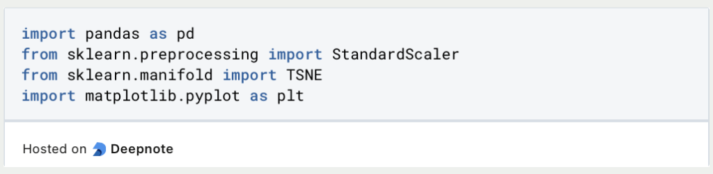
The necessary imports for this example include Pandas for working with the data set, Scikit-Learn for scaling the data and for dimensionality reduction with t-SNE, as well as matplotlib so that the two-dimensional data can also be visualized afterwards.

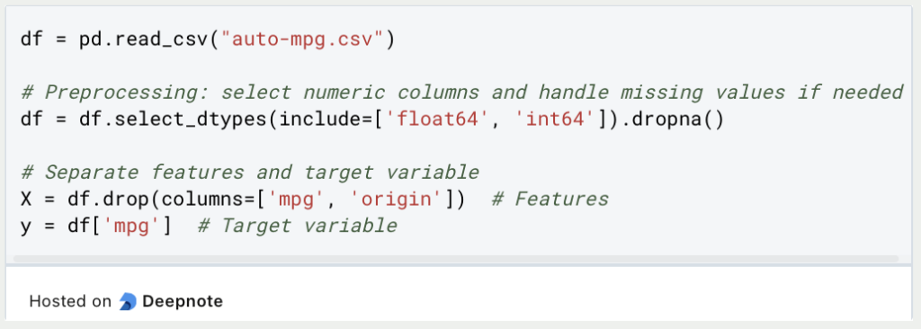
The data set is loaded from a CSV file and the categorical variable origin is then removed, as this cannot be easily processed by t-SNE. In addition, the information on miles per gallon (MPG) is removed, as this should not be included in the reduction. t-SNE is in many cases a pre-processing step for training a machine learning model. For this, MPG would serve as a target variable and should therefore not be reduced.

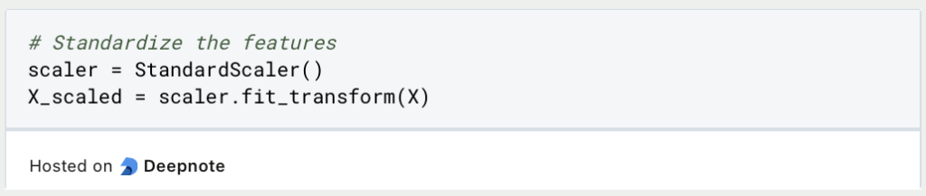
Before applying the t-SNE algorithm to the data, it is a good idea to scale the dimensions to a uniform value, for example between 0 and 1. Although this is not a necessary step, it can have beneficial effects on the training process so that dimensions with higher scales are not favored in the dimensionality reduction only because of the higher scale. In addition, t-SNE can also converge faster with scaled dimensions.

There are many ways to scale the data set. In this example, the standard scaler is used.

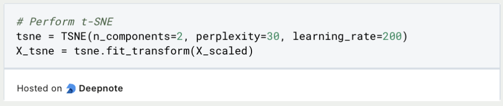
The t-SNE variable is then instantiated with the hyperparameters. This determines the number of components, i.e. the number of dimensions that the result should have. The learning rate specifies how large the steps between the iterations should be and the perplexity determines the influence of nearby points on the probability compared to distant points.

The results from the training process of t-SNE can now be visualized in a two-dimensional diagram. It is important to note that the two dimensions no longer have anything to do with the original dimensions and therefore cannot be named directly, as they represent a mixture of the previously used dimensions.

This is what you should take with you

• t-distributed stochastic neighbor embedding (tSNE for short) is an unsupervised algorithm for dimension reduction in large data sets.
• It is used to reduce the dimension of data sets and thus prevent possible overfitting of models.
• The main difference to Principal Component Analysis is that it can also be used for non-linear relationships between the data points. This property has a far-reaching influence, for example, on the reproducibility of the results or on the computing time required.
• In Python, t-SNE can be implemented using the Scikit-Learn library, for example.

Other Articles on the Topic of tSNE

• Scikit-Learn provides extensive documentation on how to use tSNE in Python.