K-nearest neighbors (KNN for short) describes a supervised learning algorithm that uses distance calculations between points to classify data. It can assign a class to new data points by determining the k-nearest data points and applying their majority class to the new data point.

How does the algorithm work?

Classification is a general attempt to assign the points in a data set to a certain class. Accordingly, a model is to be trained that can then independently decide for new points to which class they should best belong. These models can be either in the domain of supervised or unsupervised learning. One distinguishes with it whether the training data set already has a special class assignment or not.

If, for example, we want to divide the customers of a company into three different groups depending on their purchasing power and the number of purchases, we distinguish between a supervised learning algorithm in which the customers in the training data set have already been assigned to a customer group and the model is to infer new values based on this given classification. In unsupervised learning, on the other hand, the customers in the training data set are not yet classified and the model must find groupings independently based on the recognized structures.

Suppose we take the following customers as an example to explain the KNN algorithm:

Customer	Total Sales	Count Purchases	Group
A	10.000 €	5	A
B	1.500 €	1	B
C	7.500 €	3	A

For the k-Nearest Neighbor algorithm, a concrete value for k must first be determined at the beginning. This specifies how many neighbors we will compare the new data point with in the end. For our example, we choose k = 2. Let’s assume that we now have a new customer D who has already made a purchase from us for 9,000 € and has made a total of four purchases. To determine its classification, we now search for the two (k=2) nearest neighbors to this data point and determine their class.

In our case, these are customer A and C, who both belong to class “A”. So we classify the new customer D as an A-customer as well, since its next two neighbors belong to class “A” in the majority.

Besides the choice of the value k, the distance calculation between the points determines the quality of the model. There are different calculation methods for this.

How can distances be calculated?

Depending on the use case and the characteristics of the data, various distance functions can be used to determine the nearest neighbors. We will take a closer look at these in this chapter.

Euclidean Distance

The Euclidean distance is the most widely used and can be applied to real vectors with many dimensions. It involves calculating the distances between two points in all dimensions, squaring them, and then summing them. The square root of this sum is then the final result.

\(\) \[d(x,y) = \sqrt{\sum_{i = 1}^{n}(y_{i} – x_{i})^2}\]

Simply place a direct line between the two points x and y and measure their length.

Manhattan Distance

The Manhattan distance, on the other hand, calculates the absolute difference of the points in all dimensions and is therefore also called “cab distance”. This is because the procedure is similar to the journey of a cab through the vertical streets in New York.

\(\) \[d(x,y) = \sum_{i = 1}^{n}|y_{i} – x_{i}|\]

The use of this distance function makes sense especially when you want to compare objects with each other. For example, if two houses are to be compared by looking more closely at the number of rooms and the living area in square meters, it makes no sense to take the Euclidean distance, but to look separately at the difference in the rooms and then at the difference in the living area. Otherwise, these dimensions would be confused with different units.

Other Distance Functions

In addition, there are other distance functions that can be used if you use special data formats. For example, the Hamming distance is useful for Boolean values such as True and False. The Minkowski distance, on the other hand, is a mixture of the Euclic and Manhattan distances.

Which applications use the KNN?

When working with large data sets, classifying helps to get a first impression about the feature expressions and the distribution of the data points. In addition, there are many other applications for classifying:

• Market segmentation: An attempt is made to find similar customer groups with comparable purchasing behavior or other characteristics.
• Image segmentation: An attempt is made to find the locations within an image that belongs to a specific object, e.g. all pixels that are part of a car or the road.
• Document Clustering: Within a document, an attempt is made to find passages with a similar content focus.
• Recommendation Engine: When recommending products, similar customers are searched for with the help of k-Nearest Neighbors, and their purchased products are suggested to the respective customer if he has not yet purchased them.
• Healthcare: When testing drugs and their effectiveness, KNN is used to search for particularly similar patients and then administer the drug to one patient and not to the other. This makes it possible to compare which effects were triggered by the drug and which might have occurred anyway.

What are the advantages and disadvantages of the k-Nearest Neighbor algorithm?

The k-nearest Neighbor model enjoys great popularity because it is easy to understand and apply. Moreover, there are only two hyperparameters that can be varied, namely the number of neighbors k and the distance metric. On the other hand, this is of course also a disadvantage, since the algorithm can be adapted only little or not at all to the concrete application.

However, due to its simplicity, the k-Nearest Neighbors algorithm also requires a lot of time and memory for large data sets, which quickly becomes a cost factor for larger projects. Therefore, larger data projects like to rely on more elaborate models, such as k-means clustering.

What is the difference between k-nearest neighbors and k-means?

Although the names of the k-Nearest Neighbors algorithm and k-Means clustering sound very similar at first, they have relatively little in common and are used for completely different applications. The k in k-Means Clustering describes the number of classes into which the algorithm divides a data set. In k-Nearest Neighbors, on the other hand, k stands for the number of neighbors that are used to determine the class of the new data point.

Furthermore, the k-Nearest Neighbors model is a supervised learning model, since it requires the assignment to groups to derive new ones. The k-Means clustering, on the other hand, is an unsupervised learning algorithm, since it can recognize different groups independently based on the structures in the data and assign the data to these classes.

How can you do k-nearest neighbor matching in Python?

The k-nearest neighbor matching is a helpful algorithm for classifying and finding similar data. This can be implemented relatively easily in Python, as we will show in this section using the IRIS dataset.

Step 1: Import libraries

The first step is to import the required Python libraries. We need numpy and scikit-learn from whose library we load the data set and also use the stored model for the k-nearest neighbor.

Step 2: Load a Public Dataset

In this example, we use the Iris dataset, which is a well-known and publicly available dataset for machine learning applications. It is already available in the scikit-learn library.

Step 3: Create a k-nearest neighbor Model

Once the data set has been stored, the actual model can now be created using the NereastNeighbors class. The number of neighbors to be searched for must be specified, as well as the measurement method for the distance.

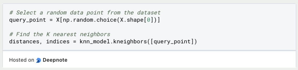
Step 4: Perform K-NN Matching

Once the model has been trained, it can be used to find the nearest neighbors for any given data point. In our example, an arbitrary point is created for this purpose and the neighbors in the data set are searched for.

Step 5: Review Results

The results from step 4 can now be output and the points of the nearest neighbors can be output:

Step 6: Interpretation and Further Analysis

In addition to the actual points, the distances to these neighbors are also returned. This makes it possible to see how close the points really are to each other. You can then decide whether an interpretation is possible or whether the points are too far apart.

Using these basic steps, a simple k-nearest neighbor algorithm can be trained and used in Python. The same principles and steps can also be applied to your own data set.

How can you improve the results of k-nearest neighbor?

K-nearest neighbor Matching is a simple algorithm that can be trained and used quickly. However, some optimizations can be made to achieve the best possible result. The following points should be decided before use:

• Optimal selection of the K value: The selection of the number of neighbors searched for is a decisive factor for good results. Too large a k can lead to distortions, while too small a k leads to noisy predictions. The ideal k can be determined using techniques such as cross-validation and thus adapted to the data set.
• Selection and construction of features: The quality of the prediction is critically dependent on the features in the dataset. The most relevant features should therefore be identified and used. In addition, feature engineering can be considered to create new features that are a combination of the existing attributes.
• Distance metrics: Distance metrics play a crucial role in nearest-neighbor searches as they influence how feature scales are interpreted. The most common distance metrics are Euclidean or Manhattan distance. It is best to experiment with different metrics to achieve the optimum result.
• Scaling of features: The different scales of numerical features can significantly affect the performance of k-NN. Therefore, these should be normalized if possible, for example with the MinMax scaler or Z-score normalization. This ensures that individual features do not have a disproportionate effect on neighbor findings.
• Data processing: If the data set contains missing values, these should be filled in, for example using techniques such as imputation. Otherwise, incorrect predictions may be made for data points with outliers or missing values.
• Weighted K-NN: The standard k-nearest neighbor matching treats all neighbors identically, no matter how close or far they are from the data point. A weighted k-NN ensures that closer neighbors have more influence on predictions. This can be useful in many applications.
• Dimension reduction: Before training the model, it can be useful to use techniques that reduce the number of dimensions, such as PCA or tSNE. This can improve the efficiency of k-nearest neighbor matching while avoiding the curse of dimensionality.

Using these strategies, a k-NN model can be customized to your specific dataset and application to improve performance and accuracy.

This is what you should take with you

• k-Nearest Neighbors is a supervised learning algorithm that uses distance calculations between data points to divide them into groups.
• A new point can be assigned to a group by looking at the k neighboring data points and using their majority class.
• Such a clustering method can be useful for navigating large data sets, making product recommendations for new customers, or dividing test and control groups in medical trials.

Other Articles on the Topic of k-Nearest Neighbors

IBM has written an interesting post on the k-Nearest Neighbor model.