The Decision Tree is a machine learning algorithm that takes its name from its tree-like structure and is used to represent multiple decision stages and the possible response paths. The decision tree provides good results for classification tasks or regression analyses.
What do we use Decision Trees for?
With the help of the tree structure, an attempt is made not only to visualize the various decision levels but also to put them in a certain order. For individual data points, predictions can be made, for example, a classification by arriving at the target value along with the observations in the branches.
The decision trees are used for classifications or regressions depending on the target variable. If the last value of the tree can be mapped to a continuous scale, we speak of a regression tree. On the other hand, if the target variable belongs to a category, we speak of a classification tree.
Due to this simple structure, this type of decision-making is very popular and is used in a wide variety of fields:
- Business management: Opaque cost structures can be illustrated with the help of a tree structure and make clear which decisions entail how many costs.
- Medicine: Decision trees are helpful for patients to find out whether they should seek medical help.
- Machine Learning and Artificial Intelligence: In this area, decision trees are used to learn classification or regression tasks and then make predictions.
Structure of a Decision Tree
A tree essentially consists of three major components: Roots, Branches, and Nodes. To better understand these components, let’s take a closer look at an example tree that helps us decide whether or not to exercise outside today.
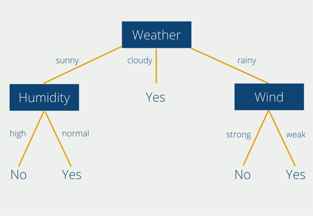
The top node “Weather” is the so-called root node, which is used as the basis for the decision. Decision trees always have exactly one root node, so that the entry point for all decisions is the same. At this node hang the so-called branches with the decision possibilities. In our case, the weather can be either cloudy, sunny, or rainy. Two of the branches (“sunny” and “rainy”) hang so-called nodes. At these points, a new decision has to be made. Only the branch “cloudy” leads directly to a result (leaf). So from our tree, we can already read that we should always go outside for sports when the weather is cloudy.
In sunny or rainy weather, on the other hand, we have to consider a second component, depending on our weather result. For the node “Humidity” we can choose between “high” and “normal”. If the humidity is high, we end up with the “No” leaf. In sunny weather paired with high humidity, it is therefore not advisable to do sports outside.
If the weather is rainy, we are in another branch within our decision tree. Then we have to make a decision at the node “wind”. The decision options here are “strong” or “weak”. Again, we can read two rules: If it is raining but the wind is weak, we can do sports outside. If it is raining coupled with strong wind, on the other hand, we should stay at home.
This very simple example can of course be further extended and refined. For the nodes “humidity” and “wind”, for example, one could consider replacing the subjective decision options with concrete rules (strong wind = wind speeds > 10 kmh) or subdividing the branches even more finely.
What is the so-called Pruning?
Decision trees can quickly become complex and confusing in real-world use cases since in most scenarios more than two decisions are needed to end up with one result. To prevent this, trained decision trees are often pruned.
Reduced error pruning is a bottom-up algorithm that starts at the leaves and gradually works its way to the root. This involves taking the entire decision tree and leaving out one node including the decisions. Then, a comparison is made to see if the prediction accuracy of the truncated tree has deteriorated. If this is not the case, the tree is shortened by this node and the complexity of the decision tree is reduced.
In addition to the possibility of shortening the tree after the training, there are also methods to keep the complexity low already before or during the training. A popular algorithm for this is the so-called early stopping rule. During training, a decision is made after each created node as to whether the tree is to be continued at this point, i.e. whether it is a decision node, or whether it is a result node. In many cases, the so-called Gini Impurity is used as a criterion.
Simply put, it expresses the probability that a label will be set incorrectly at this node if it is simply assigned randomly, i.e. based on the distribution at this node. The smaller this ratio, the higher the probability that we can prune the tree at this point without having to fear large losses in the accuracy of the model.
What are the advantages and disadvantages of Decision Trees?
The simple and understandable structure makes the decision tree a popular choice in many use cases. However, the following advantages and disadvantages should be weighed before using this model.
| Advantages | Disadvantages |
| Easy to understand, interpret and visualize. | Decision Trees can be unstable and change greatly with slight changes in training data. |
| Applications with categorical values (sunny, cloudy, rainy) and numerical values (wind speed = 10 kmh) can be mapped. | In the case of unbalanced training data (e.g. very often sunny weather) this so-called bias can also be present in the tree. |
| Non-linear relationships between variables do not affect the accuracy of the tree. | Trees can quickly become very complex and overfit the training data. As a result, they do not generalize as well to previously unseen data. |
| The number of decision-making levels is theoretically unlimited. | High training time |
| Several decision trees can be combined to form a so-called random forest. |
Decision trees as part of Random Forests
Random Forest is a supervised Machine Learning algorithm that is composed of individual decision trees. Such a type of model is called an ensemble model since an “ensemble” of independent models is used to compute a result. In practice, this algorithm is used for various classification tasks or regression analyses. The advantages are the usually short training time and the traceability of the procedure.
The Random Forest consists of a large number of these decision trees, which work together as a so-called ensemble. Each individual decision tree makes a prediction, such as a classification result, and the forest uses the result supported by most of the decision trees as the prediction of the entire ensemble. Why are multiple decision trees so much better than a single one?
The secret behind the Random Forest is the so-called principle of the wisdom of many. The basic idea is that the decision of many is always better than the decision of a single individual or a single decision tree. This concept was first recognized in the estimation of a continuous set.
In 1906, an ox was shown to a total of 800 people at a fair. They were asked to estimate how heavy this ox was before it was actually weighed. It turned out that the median of the 800 estimates was only about 1% away from the actual weight of the ox. No single estimate had come that close to being correct. So the crowd as a whole had estimated better than any other single person.
This can be applied in exactly the same way to the Random Forest. A large number of decision trees and their aggregated prediction will always outperform a single decision tree.

However, this is only true if the trees are not correlated with each other and thus the errors of a single tree are compensated by other Decision Trees. Let us return to our example with the ox weight at the fair.
The median of the estimates of all 800 people only has the chance to be better than each individual person, if the participants do not talk with each other, i.e. are uncorrelated. However, if the participants discuss together before the estimation and thus influence each other, the wisdom of the many no longer occurs.
How do you train a Decision Tree in Python?
The Scikit-Learn Python module provides a variety of tools needed for data analysis, including the decision tree. Among other things, it is based on the data formats known from Numpy. To create a decision tree in Python, we use the module and the corresponding example from the documentation.
The so-called Iris Dataset is a popular training dataset for creating a classification algorithm. It is an example from biology and deals with the classification of so-called iris plants. About each flower the length and width of the petal and the so-called sepal are available. Based on these four pieces of information, it is then to be learned which of the three iris types this specific flower is.
With the help of Skicit-Learn, a decision tree can be trained in just a few lines of code:
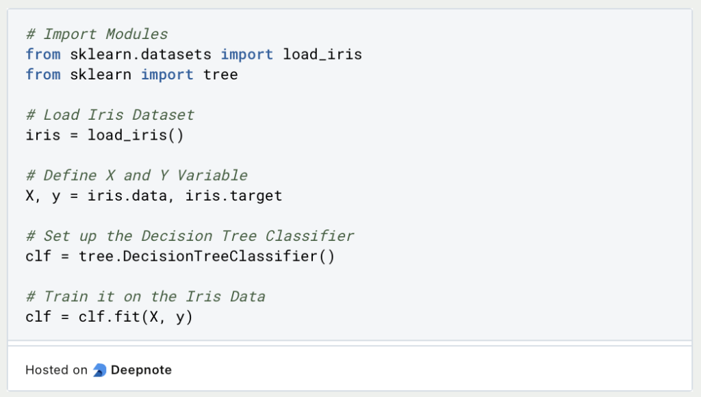
So we can train a decision tree relatively easily by defining the input variable X and the classes Y to be predicted, and training the decision tree from Skicit-Learn on them. With the function “predict_proba” and concrete values, a classification can then be made:
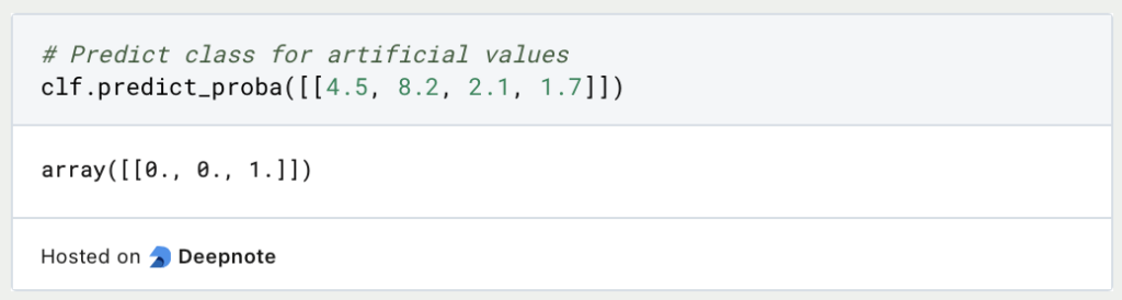
So this flower with the made-up values would belong to the first class according to our Decision Tree. This genus is called “Iris Setosa”.
How to interpret Decision Trees?
With the help of MatplotLib, the trained decision tree can be drawn.
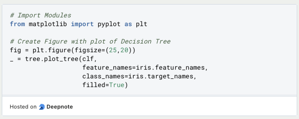
The optimal decision tree for our data has a total of five decision levels:
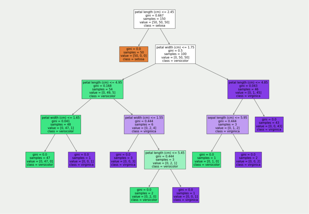
For the simple interpretation of this tree, we are interested in the value in the first and the last line. The tree is read from top to bottom. This means that in the first decision level, we check whether the length of the petal is less than or equal to 2.45 cm. The conditions are always formulated so there is only “True” in the left branch and “False” in the right branch.
So, if a concrete flower has a petal that is less than or equal to 2.45 cm, we are in the left branch (in the orange tile), which is also a result leaf. Thus we know that in this case, the flower belongs to the class “Setosa”.
If, on the other hand, the petal is longer, we go along the right branch and are faced with another decision, namely whether the petal has a maximum width of 1.75 cm. We work our way through the tree until we reach a result sheet that provides information about the classification.
This is what you should take with you
- Decision trees are another machine learning algorithm mainly used for classifications or regressions.
- A tree consists of the starting point, the so-called root, the branches representing the decision possibilities, and the nodes with the decision levels.
- To reduce the complexity and size of a tree, we apply so-called pruning methods that reduce the number of nodes.
- Decision Trees are well suited to vividly represent decision-making and make it explainable.
- However, when training, one has to pay attention to many details in order to obtain a meaningful model.
Thanks to Deepnote for sponsoring this article! Deepnote offers me the possibility to embed Python code easily and quickly on this website and also to host the related notebooks in the cloud.

What is a Boltzmann Machine?
Unlocking the Power of Boltzmann Machines: From Theory to Applications in Deep Learning. Explore their role in AI.

What is the Gini Impurity?
Explore Gini impurity: A crucial metric shaping decision trees in machine learning.

What is the Hessian Matrix?
Explore the Hessian matrix: its math, applications in optimization & machine learning, and real-world significance.

What is Early Stopping?
Master the art of Early Stopping: Prevent overfitting, save resources, and optimize your machine learning models.

What is RMSprop?
Master RMSprop optimization for neural networks. Explore RMSprop, math, applications, and hyperparameters in deep learning.

What is the Conjugate Gradient?
Explore Conjugate Gradient: Algorithm Description, Variants, Applications and Limitations.
Other Articles on the Topic of Decision Trees
- The Python Library documentation also provides detailed explanations of Decision Trees including some concrete programmed examples.

Niklas Lang
I have been working as a machine learning engineer and software developer since 2020 and am passionate about the world of data, algorithms and software development. In addition to my work in the field, I teach at several German universities, including the IU International University of Applied Sciences and the Baden-Württemberg Cooperative State University, in the fields of data science, mathematics and business analytics.
My goal is to present complex topics such as statistics and machine learning in a way that makes them not only understandable, but also exciting and tangible. I combine practical experience from industry with sound theoretical foundations to prepare my students in the best possible way for the challenges of the data world.