In machine learning, creating a good model is only the first step. Subsequently, it is at least as important to measure the predictive quality of the model and check how well it can handle new data that was not part of the training. The model evaluation comprises various processes to measure model quality and the so-called generalization capability independently. Model evaluation should be part of any training to avoid misleading predictions and ensure that the model will likely work well in the application.

In this article, we provide an overview of the various evaluation methods used within model evaluation. In addition, we also look at the different metrics used for evaluation and how they work to assess the quality of the model.

What is Model Evaluation?

Model evaluation refers to the process in machine learning during which the performance of a model is systematically checked and evaluated. The aim is to find out how good the prediction quality of the model is and how well it can be used to predict new data. The final application should be simulated during the model creation process so that it becomes clear whether it can also deliver good results in practice later on.

The creation of a model carries the risk that it will make incorrect predictions in practice, which can have far-reaching consequences, for example, if it is used to make investment decisions. Model evaluation makes it possible to check whether the model reacts just as well to new data as it did in training, thereby minimizing the risk in practice. Model evaluation pursues these goals:

• Performance Evaluation: It is important to be able to measure and compare the performance of the model with other architectures.
• Robustness: The model should not only deliver good results for the data set used in training but also in later use, where it may encounter slightly different data. The model evaluation helps to assess how robust the model will be later on.
• Generalization Capability: Model training aims to identify the underlying structures in the data so that they can be applied to new data sets. Model evaluation can be used to find out whether the model has merely memorized the data or has really understood it.

What Methods are Used in Model Evaluation?

When training machine learning models, you usually have a specific use case in mind, such as the creation of a spam classification for emails, for which the created model will later be used. At the time of training, however, you only have a training dataset that contains data from the past, which is why it is difficult to assess how well the model will behave later in the application on new, previously unseen data. It is said that the model generalizes well if it has recognized the underlying patterns in the data in the training data set so that it also performs well in the later application.

To obtain sufficient results during the creation and training of the model to determine how well the model will generalize later, two methods have been developed in the field of model evaluation that simulate the later use case by providing new data for the model.

Train/Test-Split

The train/test split is a widely used method within model evaluation that can be used after model training to determine how good the predictions are for new/unseen data. The available data is split into two parts:

• Training Data: This part of the dataset is used during training to refine the architecture of the model, i.e. to adjust parameters and recognize the underlying structures in the data.
• Test Data: These data points were not used in training and are therefore still completely new for the trained model. They are used after training for model evaluation in order to assess how the model reacts to new, unseen data and thus to simulate the real use case.

The train/test split helps to assess whether a model merely learns the training data by heart or understands the data set and recognizes the underlying patterns so that it is likely to generalize well. Without this assessment, the evaluation of performance would probably be too optimistic if the model were tested with the same data it was trained with.

This situation is also familiar in real life when you learn vocabulary in a new language, for example, 20 words. If you repeat them over and over again, i.e. learn them, then at some point, you become very good at repeating them. So if you can translate 19 out of 20 words correctly after a certain amount of training time, then you have done very well, but this result does not make it clear whether the training time was simply used to memorize the words or whether you have understood the foreign language a little better.

With the help of the train/test split, you would only use 15 vocabulary items to learn and then put them aside after the training process and look at the last five to see if you can translate them even though you have never seen them before. This then shows whether you have understood the language and recognize, for example, that you have learned the word “play” in training and can therefore now translate the word “player” in the test data set.

This method is particularly simple and can be quickly implemented in a model. Depending on the data set size, you can try different splits, such as using 90% of the data set for training and 10% for testing. However, problems can arise, especially with small data sets, if there are not enough data points left for training after the split.

Cross Validation

Cross-validation is another method for independently evaluating the generalization capability of the model. It goes beyond the pure train/test split by splitting the data set several times into training and test data sets and not just once. This usually provides more reliable results, as different data constellations are tested.

There are different variants of cross-validation for model evaluation:

• In k-fold cross-validation, the data set is split into k equally sized subsets, known as folds. The model is then trained a total of k times, with a different fold being used as the test set in each run and the remaining folds forming the training data set. Finally, the performance of the model can be evaluated using the k key figures.

• Leave-one-out cross-validation is the extreme form of this, in which each fold consists of just a single data point from the data set. The model is then always trained with the entire data set except for one data point and the performance is evaluated. Although this model evaluation method offers very reliable results, it is also very computationally intensive, which is why it should only be used for smaller data sets and simple model architectures, as otherwise, the use of resources is disproportionate to the result.

The cross-validation methods offer a robust evaluation of the model’s performance and can also be used for small data sets where the train/test split may not be suitable. They can now also be easily integrated into existing models using various machine-learning libraries.

Which Metrics are used for Model Evaluation?

In order to evaluate the performance of a model and compare it with other model architectures, special metrics are required that can be used for model evaluation. Depending on the type of application, different metrics have become widely used. In this section, we present the most popular metrics for regressions, classifications, and clusters in more detail.

Model Evaluation for Regression

Regression includes models in which continuous values are predicted, such as the price of a property or the future temperature at a certain location. In these applications, it is extremely rare for the exact correct value to be predicted, as the numerical range is simply far too large for this. Instead, the user is interested in how close the prediction comes to the actual value. This difference can be calculated using the following two key figures, for example.

Mean Absolute Error (MAE)

The mean absolute error is very easy to understand and is therefore frequently used. The absolute difference between the prediction of the model and the actual label of the data point is calculated for each data point:

\(\)\[MAE=\frac{1}{n}\sum_{i=1}^{n}{|y_i-{\hat{y}}_i|}\]

Here, \(y_i\) stands for the label of the data point \(i\) and \(\hat{y_i}\) for the prediction of the model for the corresponding data point. The main advantage of this metric is that it is easy to interpret and calculate, which is why it is mainly used when the error term of a model is to be interpreted explicitly. Mathematically, this error is advantageous because it is robust to outliers. This means that it is not sensitive to data points that differ significantly from the other data points.

A disadvantage of this key figure is that every error is treated equally and very strong deviations carry just as much weight as slight deviations.

Mean Squared Error (MSE)

The mean squared error is very similar to the key figure presented above, with the difference that the difference between the prediction and the actual result is also squared and not just the amount:

\(\)\[MSE=\frac{1}{n}\sum_{i=1}^{n}\left(y_i-{\hat{y}}_i\right)^2\]

This small difference ensures that large deviations carry more weight than small deviations, as numbers greater than one are significantly increased by the square, while small deviations less than one are reduced by the square. In addition, this function has advantageous mathematical features, such as the fact that it can be derived, which makes it interesting for many optimization algorithms.

Model Evaluation for Classification

In classification tasks, the prediction consists of correctly assigning a data point to one of two or more classes, as is done in spam detection or image classification, for example. This also results in other types of metrics that are used specifically for classifications.

In the simplest case, a classification consists of two states. Suppose we want to investigate how well corona tests reflect the infection status of a patient. In this case, the corona test serves as a classifier of a total of two states: infected or non-infected.

These two classes can result in a total of four states, depending on whether the classification of the test was correct:

• True Positive: The rapid test classifies the person as infected and a subsequent PCR test confirms this result. The rapid test was therefore correct.
• False Positive: The rapid test is positive for a person, but a subsequent PCR test shows that the person is not actually infected, i.e. negative.
• True Negative: The rapid test is negative and the person is not infected.
• False Negative: The coronavirus rapid test classifies the person tested as healthy, i.e. negative, but the person is infected and should therefore have a positive rapid test.

With the help of these cases, some interesting key figures can already be calculated. The most frequently used key figure is the accuracy, which measures how many of the predictions were correct in proportion.

\(\) \[\text{Accuracy} = \frac{\text{True Positive + True Negative}}{\text{True Positive + True Negative + False Positive + False Negative}}\]

However, this metric can be misleading, especially in unbalanced data where one class is represented more often than another.

Precision is one of the most widely used metrics when analyzing models and measures the proportion of positive predictions in a classification that were correctly classified compared to the total number of positive cases in the data set. This measures the ability to prevent false positive errors. This occurs when the model incorrectly predicts a positive result, for example, that a patient is ill, but in reality, a negative result exists, i.e. the patient is not ill.

\(\) \[\text{Precision} = \frac{\text{True Positive}}{\text{True Positive + False Positive}}\]

In the case of spam detection, on the other hand, precision measures the proportion of emails that were spam, i.e. positive, about the emails that were classified as spam by the program. This proportion is made up of the true positives, i.e. the correctly predicted positive values, and the incorrectly classified positive values. A high precision value means that a large proportion of the emails declared as spam were spam and only a few emails ended up in the spam folder by mistake. A low value, on the other hand, indicates a high number of incorrectly declared spam emails, which can lead to a high level of frustration for the user.

Another error has an indirect influence on the precision value. The false negative error occurs in cases where the machine learning model predicts a negative result, although this does not correspond to reality. In the case of a false negative error, actual spam emails would end up in the inbox because they were not recognized and were classified as normal emails. This error indirectly influences the precision, as fewer emails can be classified as true positives. This is because more true positive cases automatically mean fewer false negative cases and vice versa.

To optimize precision, it is therefore important to reduce the number of false positives while at the same time not increasing the false negatives too much and keeping them at an acceptable level. In applications where both false positives and false negatives are equally bad, looking at precision is usually not enough. Therefore, other metrics, such as recall or F1 score, should also be considered to get a more complete picture of model performance.

In machine learning, recall, or sensitivity, refers to the ability of a model to correctly predict the important instances in a data set. The ratio between the correctly predicted positive instances (true positives) and the total number of all actual positive instances (true positives + false negatives) is calculated. This key figure is also used to measure that the number of false negatives is kept within limits, which was not taken into account in the precision.

\(\) \[\text{Recall} = \frac{\text{True Positives} }{\text{True Positives + False Negatives}}\]

Recall is particularly important in applications where the focus is on identifying all positive instances and where false predictions can also be accepted. In medicine, for example, it is more important to recognize all sick people, even if this means that a few healthy people may be incorrectly classified as sick. However, if a sick patient is not recognized, this can have much more serious consequences than mistakenly treating a healthy person.

The sensitivity assumes values between 0 and 1, where 1 stands for a model that correctly predicts all positive data points as positive. Zero, on the other hand, means that the model has not correctly identified a single positive instance in the data set.

The F1 score is a popular indicator for the evaluation of binary classification models and represents the harmonic mean of precision and recall. It is particularly useful if both metrics are to be weighted equally. It is calculated as the ratio of twice the product of precision and recall divided by their sum:

\(\) \[\text{F1} = \frac{2 \cdot \text{Precision} \cdot \text{Recall}}{\text{Precision + Recall}}\]

This score can take values between 0 and 1, with a high value indicating good model performance with high precision and high recall. This metric is particularly useful when the data set is unbalanced and there is a risk that the model is biased towards the more frequent class. In applications such as medicine or fraud detection in the financial sector, healthy people or normal transactions occur much more frequently and are therefore also represented in the majority of data sets. However, to prevent the model from developing a tendency to frequently classify the data points as healthy people or normal transactions, the F1 score is used to account for this imbalance.

Model Evaluation for Clustering

The clustering process aims to divide the data points into different groups so that all points in one group are as similar as possible to each other and at the same time as different as possible from the data points in other groups. The following metrics are mainly used for this:

Silhouette Score

This key figure calculates the similarity of a data point to its cluster and compares this with the similarity of the data point to another data cluster. The following calculations are performed for each data point:

• \(a(i)\) is the average distance of the data point \(i\) to all other points in the same cluster, i.e. the so-called intra-cluster distance.
• \(b(i)\) is the average distance of the data point \(i\) to all data points in the nearest cluster, i.e. the inter-cluster distance.

With the help of these two components, the silhouette score is then calculated as follows:

\(\)\[s(i) = \frac{b(i) – a(i)}{max(a(i), b(i))}\]

The values are then between -1 and 1, with a value close to -1 indicating that the specific data point may have been assigned to an incorrect cluster. Accordingly, a value close to 1 means that the data point is assigned to the correct cluster and a value around 0 indicates that the point lies on the boundary between two neighboring clusters.

Adjusted Rand Index (ARI)

This index can be used in model evaluation if a so-called ground-truth cluster assignment exists, i.e. a label in the data set already clarifies for each data point which class the data point should be assigned to. Similar to classification, the predicted clusters can then be compared with the actual clusters, and a key figure is determined based on this. Random data pairs are selected and it is then determined whether they were either correctly assigned to the same cluster or whether they were correctly assigned to different clusters. The ARI then uses this to compare whether the model behaves better than a random allocation of clusters.

How can the Generalization Ability of a Model be evaluated?

The generalization ability of a model is the ability to recognize the underlying structures in the data and thus make good predictions with new, unknown data. This means that the model works not only on the training data but also in real applications. There are two widely used methods for testing the generalization capability.

Train-test Gap

The train-test gap describes the deviation between the model performance on the training data and the performance on the test data. The test data was a part of the data set that was explicitly not used for training so that data is available for testing that the model has not yet seen.

A small train-test gap in the model evaluation indicates that the model performs about equally well on the training data as on the test data. It can therefore be assumed that the model has generalized well overall and has not just memorized the training data.

On the other hand, a large train-test gap is problematic as there are large differences between the model performance. This can be for one of two reasons:

• Overfitting occurs when the model has only memorized the training data and therefore provides good metrics on the training data, but poor results for the test data.

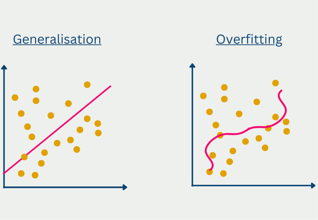
• Underfitting, on the other hand, occurs when the model architecture is simply too simple to recognize and map the complex structures in the data. In such a case, the discrepancy between training and test in the model evaluation may not be so large, but the performance on both data sets is very poor.

Strategies such as regularization or better hyperparameter tuning can help avoid overfitting by reducing the discrepancy between the training and test datasets and creating a model that can generalize well.

Out-of-Sample Testing

Out-of-sample testing goes beyond the classic train-test gap by adding data that the model has not seen in either the training data set or the validation data set. It is important to note that this also involves data that varies slightly from the data set, i.e. that was taken from a slightly different data distribution.

Depending on the application, data sets can be used that were collected at a different time or in a different region, for example, so that they have slightly different characteristics. A powerful model should be able to provide good predictions even for such deviating data, and the performance should not differ greatly from the results of the test data set. If there is a significant drop in performance, this is an indicator that the model may have overfitted and adjusted too much to the characteristics of the training data set.

This is what you should take with you

• Model evaluation is the process used to assess how well a machine learning model is performing.
• To be able to recognize whether the model has merely memorized the training data or has recognized structures, you can either use the train/test split in model evaluation or rely on cross-validation to withhold part of the data set and thus be able to evaluate the performance of the model independently.
• Depending on the application, the model evaluation uses various key figures for the areas of regression, classification, and clustering.
• To evaluate the generalization ability of the model, you can either calculate the gap between the performance on the training and test data set or use an out-of-sample method.

Other Articles on the Topic of Model Evaluation

You can find a detailed article on how to do Model Evaluation in Scikit-Learn here.