Recurrent Neural Networks (RNNs) are the third major type of neural network, along with Feedforward Networks and Convolutional Neural Networks. They are used with time series data and sequential information, i.e. data where the previous data point influences the current one. These networks contain at least one recurrent layer. In this article, we will take a closer look at what this means.

What are Recurrent Neural Networks?

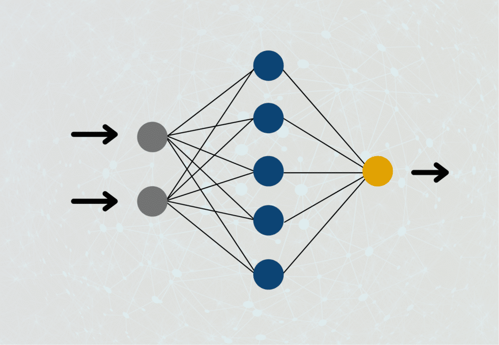
To understand how Recurrent Neural Networks work, we have to take another look at how normal feedforward neural networks are structured. In these, a neuron of the hidden layer is connected with the neurons from the previous layer and the neurons from the following layer. In such a network, the output of a neuron can only be passed forward, but never to a neuron on the same layer or even the previous layer, hence the name “feedforward”.

This is different for recurrent neural networks. The output of a neuron can very well be used as input of a previous layer or the current layer. This is much closer to the way our brain works than the structure of feedforward neural networks. In many applications, we also need an understanding of the steps computed immediately before improving the overall result.

What are the applications of RNNs?

Recurrent Neural Networks are mainly used in natural language processing or time-series data, i.e. when the information from the immediate past plays a major role. When translating texts, we should also keep the previously processed sequence of words in the “memory” of the neural network, instead of only translating word by word independently.

As soon as we have a proverb or idiom in the text to be translated, we must also take the preceding words into account, since this is the only way we can recognize that it is a proverb. If the applications in language processing become more complex, the context is of even greater importance. For example, when we want to gather information about a specific person across a text.

Which types of RNNs are there?

Depending on how far back the output of a neuron is passed within the network, we distinguish a total of four different types of recurrent neural networks:

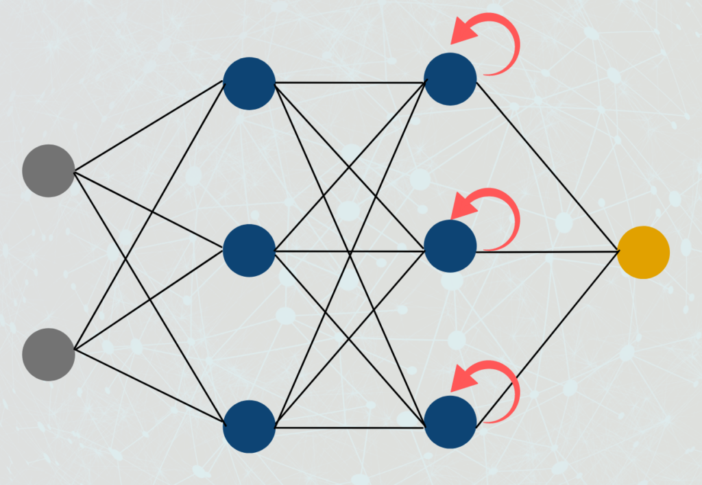
1. Direct-Feedback-Network: The output of a neuron is used as the input of the same neuron.

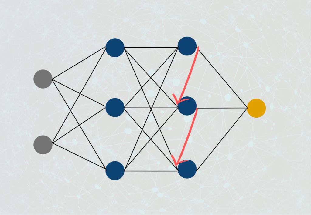
2. Indirect-Feedback-Network: The output of a neuron is used as input in one of the previous layers.

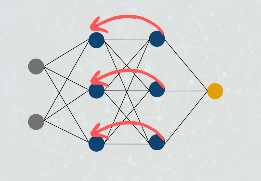
3. Lateral-Feedback-Network: Here, the output of a neuron is connected to the input of a neuron of the same layer.

4. Complete-Feedback-Network: The output of a neuron has connections to the inputs of all (!) neurons in the network, whether in the same layer, a previous layer, or a subsequent layer.

How do you train recurrent neural networks?

The training of recurrent neural networks is comparable to the training of other neural networks. In addition to data preprocessing, the initialization of the network also plays an important role in the selection of the number and structure of the layers. Compared to conventional feedforward networks, the type of RNN cells plays a decisive role, as described earlier in this article.

During the training process, a normal backpropagation takes place in which the loss of the network is first calculated during a forward pass of the model and then propagated backward through the network. The output is calculated at each time step. The partial derivative of the loss is then calculated according to the weights so that these can be adjusted accordingly to further increase the accuracy of the model. In an RNN, stochastic gradient descent is usually used as an optimization algorithm to reduce the computational complexity of the model and thus enable faster training.

However, the gradients can become vanishingly small during training, which means that the neuron weights adapt very little or not at all and the model does not continue to learn. To overcome this problem, gradient clipping can be used, in which the gradient values are limited so that they do not become too large or too small. In addition, other RNN cells can be used, such as LSTM, which can store information over longer periods.

The training of the model can be further improved by correctly setting important hyperparameters, such as the learning rate, the batch size, or the number of training epochs. As with other neural networks, random or grid search is used to find the optimal values.

Finally, it should be checked that the model is not overfitted and therefore only provides poor predictions on new, unseen data. To this end, sufficient data should be kept for a validation set to be able to evaluate the performance of the model independently and, for example, to introduce an early stopping rule that prevents overfitting at an early stage by aborting the training.

What are the problems with Recurrent Neural Networks?

Recurrent Neural Networks were a real breakthrough in the field of Deep Learning, as for the first time, the computations from the recent past were also included in the current computation, significantly improving the results in language processing. Nevertheless, during training, they also bring some problems that need to be taken into account.

As we have already explained in our article on the gradient method, when training neural networks with the gradient method, it can happen that the gradient either takes on very small values close to 0 or very large values close to infinity. In both cases, we cannot change the weights of the neurons during backpropagation, because the weight either does not change at all or we cannot multiply the number with such a large value at all. Because of the many interconnections in the recurrent neural network and the slightly modified form of the backpropagation algorithm used for it, the probability that these problems will occur is much higher than in normal feedforward networks.

Regular RNNs are very good at remembering contexts and incorporating them into predictions. For example, this allows the RNN to recognize that in the sentence “The clouds are in the ___” the word “sky” is needed to correctly complete the sentence in that context. In a longer sentence, on the other hand, it becomes much more difficult to maintain context. In the case of the slightly modified sentence “The clouds, which partly flow into each other and hang low, are in the “, it is already significantly more difficult for a Recurrent Neural Network to infer the word “sky”.

What are Long Short-Term Memory (LSTM) Models?

The problem with Recurrent Neural Networks is that they have a short-term memory to retain previous information in the current neuron. However, this ability decreases very quickly for longer sequences. As a remedy for this, the LSTM models were introduced to be able to retain past information even longer.

The problem with Recurrent Neural Networks is that they simply store the previous data in their “short-term memory”. Once the memory in it runs out, it simply deletes the longest retained information and replaces it with new data. The LSTM model attempts to escape this problem by retaining selected information in long-term memory. This long-term memory is stored in the so-called Cell State. In addition, there is also the hidden state, which we already know from normal neural networks and in which short-term information from the previous calculation steps is stored. The hidden state is the short-term memory of the model. This also explains the name Long Short-Term Networks.

In each computational step, the current input x(t) is used, the previous state of short-term memory c(t-1) and the previous state of hidden state h(t-1).

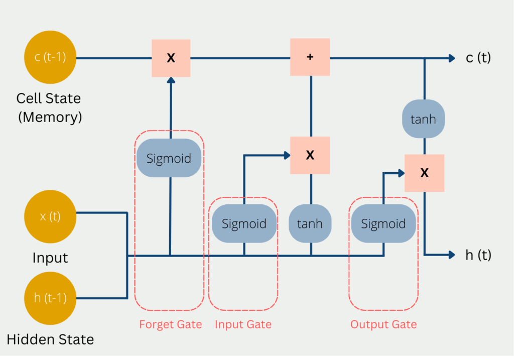
These three values pass through the following gates on their way to a new Cell State and Hidden State:

1. In the so-called Forget Gate, it is decided which current and previous information is kept and which is thrown out. This includes the hidden status from the previous pass and the current input. These values are passed into a sigmoid function, which can only output values between 0 and 1. The value 0 means that previous information can be forgotten because there is possibly new, more important information. The number one means accordingly that the previous information is preserved. The results from this are multiplied by the current Cell State, so that knowledge that is no longer needed is forgotten since it is multiplied by 0 and thus dropped out.
2. In the Input Gate, it is decided how valuable the current input is to solve the task. For this, the current input is multiplied by the hidden state and the weight matrix of the last run. All information that appears important in the Input Gate is then added to the Cell State and forms the new Cell State c(t). This new Cell State is now the current state of the long-term memory and will be used in the next run.
3. In the Output Gate, the output of the LSTM model is then calculated in the Hidden State. Depending on the application, it can be, for example, a word that complements the meaning of the sentence. To do this, the sigmoid function decides what information can come through the output gate and then the cell state is multiplied after it is activated with the tanh function.

LSTM and RNN vs. Transformer

Recurrent Neural Networks are very old by Machine Learning standards and were first introduced back in 1986. For a long time, they, and in particular the LSTM architecture were the nonplus ultra in the field of language processing to maintain context. However, since 2017 and the introduction of Transformer models and Attention Masks, this position has fundamentally changed.

The transformers differ fundamentally from previous models in that they do not process texts word for word, but consider entire sections as a whole. Thus they have clear advantages to understand contexts better. Thus, the problems of short and long-term memory, which were partially solved by LSTMs, are no longer present, because if the sentence is considered as a whole anyway, there are no problems that dependencies could be forgotten.

In addition, transformers are bidirectional in computation, which means that when processing words, they can also include the immediately following and previous words in the computation. Classical RNN or LSTM models cannot do this, since they work sequentially and thus only preceding words are part of the computation. This disadvantage was tried to avoid with so-called bidirectional RNNs, however, these are clearly more computationally expensive than transformers.

However, the bidirectional Recurrent Neural Networks still have small advantages over the transformers because the information is stored in so-called self-attention layers. With every token more to be recorded, this layer becomes harder to compute and thus increases the required computing power. This increase in effort, on the other hand, does not exist to this extent in bidirectional RNNs.

This is what you should take with you

• Recurrent Neural Networks differ from Feedforward Neural Networks in that the output of neurons is also used as input in the same or previous layers.
• They are particularly useful in language processing and for time series data when the past context should be taken into account.
• We distinguish different types of RNNs, namely direct feedback, indirect feedback, lateral feedback, or full feedback.

Other Articles on the Topic of Recurrent Neural Networks

• More information about RNNs can be found on the Tensorflow page.